第 57 章 多层线性模型
57.1 分组数据
在实验设计和数据分析中,我们可能经常会遇到分组的数据结构。所谓的分组,就是每一次观察,属于某个特定的组,比如考察学生的成绩,这些学生属于某个班级,班级又属于某个学校。有时候发现这种分组的数据,会给数据分析带来很多有意思的内容。
57.2 案例
我们从一个有意思的案例开始。
不同院系教职员工的收入
一般情况下,不同的院系,制定教师收入的依据和标准可能是不同的。我们假定有一份大学教职员的收入清单,这个学校包括信息学院、外国语学院、社会政治学、生物学院、统计学院共五个机构,我们通过数据建模,探索这个学校的薪酬制定规则。
create_data <- function() {
  df <- tibble(
    ids = 1:100,
    department = rep(c("sociology", "biology", "english", "informatics", "statistics"), 20),
    bases = rep(c(40000, 50000, 60000, 70000, 80000), 20) * runif(100, .9, 1.1),
    experience = floor(runif(100, 0, 10)),
    raises = rep(c(2000, 500, 500, 1700, 500), 20) * runif(100, .9, 1.1)
  )


  df <- df %>% mutate(
    salary = bases + experience * raises
  )
  df
}
library(tidyverse)
library(lme4)
library(modelr)
library(broom)
library(broom.mixed)

df <- create_data()
df
## # A tibble: 100 × 6
## ids department bases experience raises salary
## <int> <chr> <dbl> <dbl> <dbl> <dbl>
## 1 1 sociology 38095. 0 1809. 38095.
## 2 2 biology 47619. 2 529. 48678.
## 3 3 english 65754. 6 530. 68935.
## 4 4 informatics 72754. 4 1547. 78942.
## 5 5 statistics 79421. 5 534. 82090.
## 6 6 sociology 43379. 0 2053. 43379.
## 7 7 biology 46132. 4 484. 48069.
## 8 8 english 54064. 2 463. 54989.
## 9 9 informatics 68925. 5 1852. 78185.
## 10 10 statistics 74486. 9 533. 79284.
## # ℹ 90 more rows57.3 线性模型
薪酬制定规则一:假定教师收入主要取决于他从事工作的时间,也就说说工作时间越长收入越高。意味着,每个院系的起始薪酬(起薪)是一样的,并有相同的年度增长率。那么,这个收入问题就是一个简单线性模型:
\[\hat{y} = \alpha + \beta_1x_1 + ... + \beta_nx_n\]
具体到我们的案例中,薪酬模型可以写为 \[ \hat{salary_i} = \alpha + \beta * experience_i \]
通过这个等式,可以计算出各个系数,即截距\(\alpha\)就是起薪,斜率\(\beta\)就是年度增长率。确定了斜率和截距,也就确定了每个教职员工的收入曲线。
# Model without respect to grouping
m1 <- lm(salary ~ experience, data = df)
m1
##
## Call:
## lm(formula = salary ~ experience, data = df)
##
## Coefficients:
## (Intercept) experience
## 60572.6 820.5
broom::tidy(m1)## # A tibble: 2 × 5
## term estimate std.error statistic p.value
## <chr> <dbl> <dbl> <dbl> <dbl>
## 1 (Intercept) 60573. 2499. 24.2 3.51e-43
## 2 experience 821. 467. 1.76 8.22e- 2
df %>% modelr::add_predictions(m1)## # A tibble: 100 × 7
## ids department bases experience raises salary pred
## <int> <chr> <dbl> <dbl> <dbl> <dbl> <dbl>
## 1 1 sociology 38095. 0 1809. 38095. 60573.
## 2 2 biology 47619. 2 529. 48678. 62214.
## 3 3 english 65754. 6 530. 68935. 65496.
## 4 4 informatics 72754. 4 1547. 78942. 63855.
## 5 5 statistics 79421. 5 534. 82090. 64675.
## 6 6 sociology 43379. 0 2053. 43379. 60573.
## 7 7 biology 46132. 4 484. 48069. 63855.
## 8 8 english 54064. 2 463. 54989. 62214.
## 9 9 informatics 68925. 5 1852. 78185. 64675.
## 10 10 statistics 74486. 9 533. 79284. 67957.
## # ℹ 90 more rows
# Model without respect to grouping
df %>%
  add_predictions(m1) %>%
  ggplot(aes(x = experience, y = salary)) +
  geom_point() +
  geom_line(aes(x = experience, y = pred)) +
  labs(x = "Experience", y = "Predicted Salary") +
  ggtitle("linear model Salary Prediction") +
  scale_colour_discrete("Department")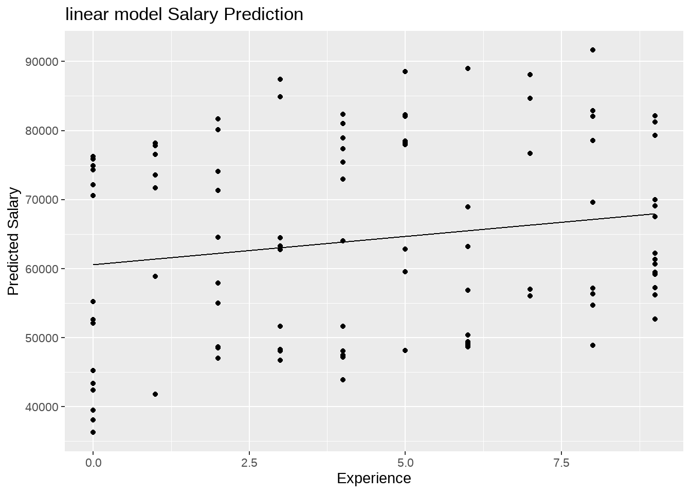
注意到,对每个教师来说,不管来自哪个学院的,系数\(\alpha\)和\(\beta\)是一样的,是固定的,因此这种简单线性模型也称之为固定效应模型。
事实上,这种线性模型的方法太过于粗狂,构建的线性直线不能反映收入随院系的变化。
57.4 变化的截距
薪酬制定规则二,假定不同的院系起薪不同,但年度增长率是相同的。
这种统计模型,相比于之前的固定效应模型(简单线性模型)而言,加入了截距会随所在学院不同而变化的思想,统计模型写为
\[\hat{y_i} = \alpha_{j[i]} + \beta x_i\]
这个等式中,斜率\(\beta\)代表着年度增长率,是一个固定值,也就前面说的固定效应项,而截距\(\alpha\)代表着起薪,随学院变化,是五个值,因为一个学院对应一个,称之为变化效应项(也叫随机效应项)。这里模型中既有固定效应项又有变化效应项,因此称之为混合效应模型。
教师\(i\),他所在的学院\(j\),记为\(j[i]\),那么教师\(i\)所在学院\(j\)对应的\(\alpha\),很自然的记为\(\alpha_{j[i]}\)
# Model with varying intercept
m2 <- lmer(salary ~ experience + (1 | department), data = df)
m2
## Linear mixed model fit by REML ['lmerMod']
## Formula: salary ~ experience + (1 | department)
## Data: df
## REML criterion at convergence: 1925.524
## Random effects:
## Groups Name Std.Dev.
## department (Intercept) 15196
## Residual 3747
## Number of obs: 100, groups: department, 5
## Fixed Effects:
## (Intercept) experience
## 59333 1102
broom.mixed::tidy(m2, effects = "fixed")## # A tibble: 2 × 5
## effect term estimate std.error statistic
## <chr> <chr> <dbl> <dbl> <dbl>
## 1 fixed (Intercept) 59333. 6828. 8.69
## 2 fixed experience 1102. 126. 8.78
broom.mixed::tidy(m2, effects = "ran_vals")## # A tibble: 5 × 6
## effect group level term estimate std.error
## <chr> <chr> <chr> <chr> <dbl> <dbl>
## 1 ran_vals department biology (Intercept) -13156. 837.
## 2 ran_vals department english (Intercept) -2103. 837.
## 3 ran_vals department informatics (Intercept) 13671. 837.
## 4 ran_vals department sociology (Intercept) -15866. 837.
## 5 ran_vals department statistics (Intercept) 17455. 837.
df %>%
  add_predictions(m2) %>%
  ggplot(aes(
    x = experience, y = salary, group = department,
    colour = department
  )) +
  geom_point() +
  geom_line(aes(x = experience, y = pred)) +
  labs(x = "Experience", y = "Predicted Salary") +
  ggtitle("Varying Intercept Salary Prediction") +
  scale_colour_discrete("Department")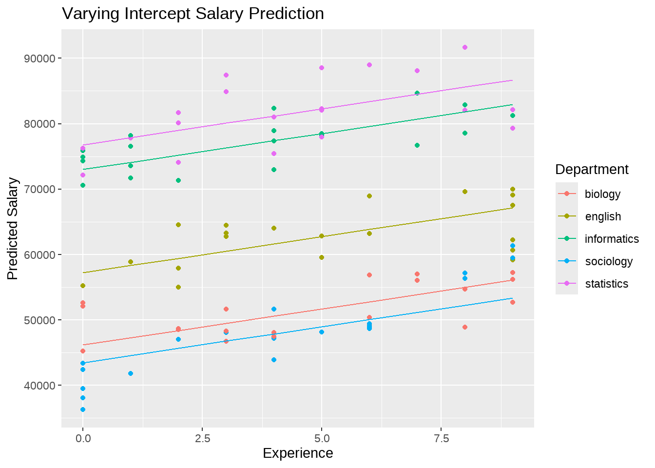
这种模型,我们就能看到院系不同 带来的员工收入的差别。
57.5 变化的斜率
薪酬制定规则三,不同的院系起始薪酬是相同的,但年度增长率不同。
与薪酬模型规则二的统计模型比较,我们只需要把变化的截距变成变化的斜率,那么统计模型可写为
\[\hat{y_i} = \alpha + \beta_{j[i]}x_i\]
这里,截距(\(\alpha\))对所有教师而言是固定不变的,而斜率(\(\beta\))会随学院不同而变化,5个学院对应着5个斜率。
# Model with varying slope
m3 <- lmer(salary ~ experience + (0 + experience | department), data = df)
m3
## Linear mixed model fit by REML ['lmerMod']
## Formula: salary ~ experience + (0 + experience | department)
## Data: df
## REML criterion at convergence: 2095.603
## Random effects:
## Groups Name Std.Dev.
## department experience 2297
## Residual 9340
## Number of obs: 100, groups: department, 5
## Fixed Effects:
## (Intercept) experience
## 59574 1146
broom.mixed::tidy(m3, effects = "fixed")## # A tibble: 2 × 5
## effect term estimate std.error statistic
## <chr> <chr> <dbl> <dbl> <dbl>
## 1 fixed (Intercept) 59574. 1649. 36.1
## 2 fixed experience 1146. 1073. 1.07
broom.mixed::tidy(m3, effects = "ran_vals")## # A tibble: 5 × 6
## effect group level term estimate std.error
## <chr> <chr> <chr> <chr> <dbl> <dbl>
## 1 ran_vals department biology experience -2099. 363.
## 2 ran_vals department english experience -440. 342.
## 3 ran_vals department informatics experience 2027. 443.
## 4 ran_vals department sociology experience -2158. 403.
## 5 ran_vals department statistics experience 2670. 397.
df %>%
  add_predictions(m3) %>%
  ggplot(aes(
    x = experience, y = salary, group = department,
    colour = department
  )) +
  geom_point() +
  geom_line(aes(x = experience, y = pred)) +
  labs(x = "Experience", y = "Predicted Salary") +
  ggtitle("Varying slope Salary Prediction") +
  scale_colour_discrete("Department")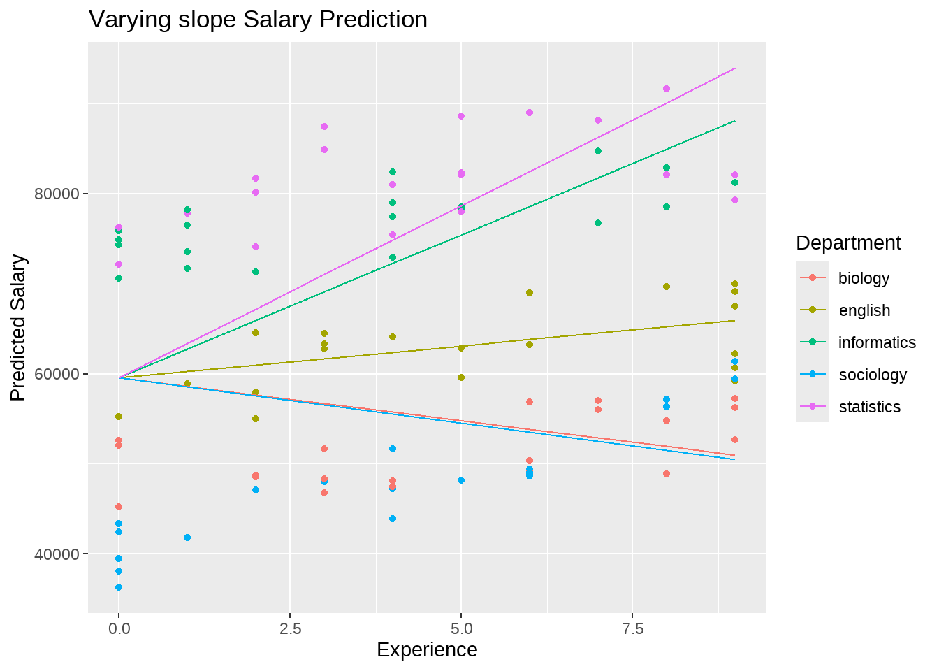
57.6 变化的斜率 + 变化的截距
薪酬制定规则四,不同的学院起始薪酬和年度增长率也不同。
这可能是最现实的一种情形了,它实际上是规则二和规则三的一种组合,要求截距和斜率都会随学院的不同变化,数学上记为
\[\hat{y_i} = \alpha_{j[i]} + \beta_{j[i]}x_i\] 具体来说,教师\(i\),所在的学院\(j\), 他的入职的起始收入表示为 (\(\alpha_{j[i]}\)),年度增长率表示为(\(\beta_{j[i]}\)).
# Model with varying slope and intercept
m4 <- lmer(salary ~ experience + (1 + experience | department), data = df)
m4
## Linear mixed model fit by REML ['lmerMod']
## Formula: salary ~ experience + (1 + experience | department)
## Data: df
## REML criterion at convergence: 1918.644
## Random effects:
## Groups Name Std.Dev. Corr
## department (Intercept) 16136.9
## experience 452.5 -0.58
## Residual 3524.3
## Number of obs: 100, groups: department, 5
## Fixed Effects:
## (Intercept) experience
## 59457 1088
broom.mixed::tidy(m4, effects = "fixed")## # A tibble: 2 × 5
## effect term estimate std.error statistic
## <chr> <chr> <dbl> <dbl> <dbl>
## 1 fixed (Intercept) 59457. 7244. 8.21
## 2 fixed experience 1088. 234. 4.64
broom.mixed::tidy(m4, effects = "ran_vals")## # A tibble: 10 × 6
## effect group level term estimate std.error
## <chr> <chr> <chr> <chr> <dbl> <dbl>
## 1 ran_vals department biology (Intercept) -12255. 1318.
## 2 ran_vals department english (Intercept) -1228. 1383.
## 3 ran_vals department informatics (Intercept) 14272. 1116.
## 4 ran_vals department sociology (Intercept) -18827. 1177.
## 5 ran_vals department statistics (Intercept) 18038. 1300.
## 6 ran_vals department biology experience -195. 218.
## 7 ran_vals department english experience -176. 217.
## 8 ran_vals department informatics experience -189. 219.
## 9 ran_vals department sociology experience 707. 213.
## 10 ran_vals department statistics experience -147. 232.
df %>%
  add_predictions(m4) %>%
  ggplot(aes(
    x = experience, y = salary, group = department,
    colour = department
  )) +
  geom_point() +
  geom_line(aes(x = experience, y = pred)) +
  labs(x = "Experience", y = "Predicted Salary") +
  ggtitle("Varying Intercept and Slopes Salary Prediction") +
  scale_colour_discrete("Department")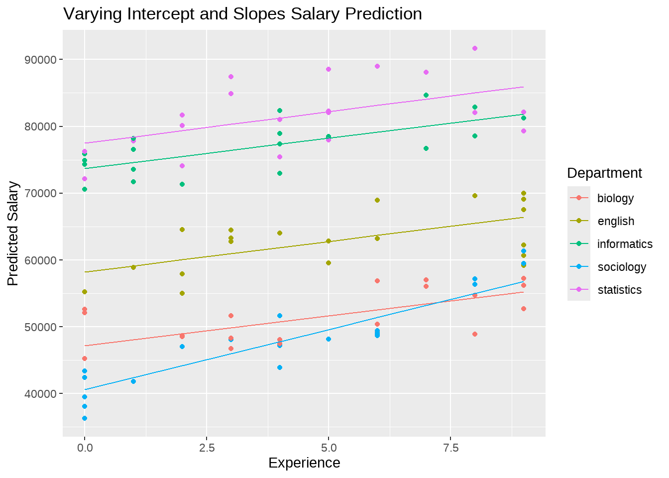
57.7 信息池
57.7.1 提问
问题:薪酬制定规则四中,不同的院系起薪不同,年度增长率也不同,我们得出了5组不同的截距和斜率,那么是不是可以等价为,先按照院系分5组,然后各算各的截距和斜率? 比如
df %>%
  group_by(department) %>%
  group_modify(
    ~ broom::tidy(lm(salary ~ 1 + experience, data = .))
  )
## # A tibble: 10 × 6
## # Groups: department [5]
## department term estimate std.error statistic p.value
## <chr> <chr> <dbl> <dbl> <dbl> <dbl>
## 1 biology (Intercept) 47938. 1332. 36.0 3.19e-18
## 2 biology experience 727. 235. 3.10 6.21e- 3
## 3 english (Intercept) 58657. 1686. 34.8 5.81e-18
## 4 english experience 826. 279. 2.96 8.43e- 3
## 5 informatics (Intercept) 73741. 1004. 73.4 9.24e-24
## 6 informatics experience 906. 217. 4.18 5.61e- 4
## 7 sociology (Intercept) 39821. 1001. 39.8 5.38e-19
## 8 sociology experience 1991. 196. 10.1 7.12e- 9
## 9 statistics (Intercept) 77298. 1968. 39.3 6.73e-19
## 10 statistics experience 998. 379. 2.63 1.70e- 2分组各自回归,与这里的(变化的截距+变化的斜率)模型,不是一回事。
57.7.2 信息共享
- 完全共享
broom::tidy(m1)## # A tibble: 2 × 5
## term estimate std.error statistic p.value
## <chr> <dbl> <dbl> <dbl> <dbl>
## 1 (Intercept) 60573. 2499. 24.2 3.51e-43
## 2 experience 821. 467. 1.76 8.22e- 2
complete_pooling <-
  broom::tidy(m1) %>%
  dplyr::select(term, estimate) %>%
  tidyr::pivot_wider(
    names_from = term,
    values_from = estimate
  ) %>%
  dplyr::rename(Intercept = `(Intercept)`, slope = experience) %>%
  dplyr::mutate(pooled = "complete_pool") %>%
  dplyr::select(pooled, Intercept, slope)

complete_pooling
## # A tibble: 1 × 3
## pooled Intercept slope
## <chr> <dbl> <dbl>
## 1 complete_pool 60573. 821.- 部分共享
fix_effect <- broom.mixed::tidy(m4, effects = "fixed")
fix_effect
fix_effect$estimate[1]
fix_effect$estimate[2]
var_effect <- broom.mixed::tidy(m4, effects = "ran_vals")
var_effect
# random effects plus fixed effect parameters
partial_pooling <- var_effect %>%
  dplyr::select(level, term, estimate) %>%
  tidyr::pivot_wider(
    names_from = term,
    values_from = estimate
  ) %>%
  dplyr::rename(Intercept = `(Intercept)`, estimate = experience) %>%
  dplyr::mutate(
    Intercept = Intercept + fix_effect$estimate[1],
    estimate = estimate + fix_effect$estimate[2]
  ) %>%
  dplyr::mutate(pool = "partial_pool") %>%
  dplyr::select(pool, level, Intercept, estimate)

partial_pooling
partial_pooling <-
  coef(m4)$department %>%
  tibble::rownames_to_column() %>%
  dplyr::rename(level = rowname, Intercept = `(Intercept)`, slope = experience) %>%
  dplyr::mutate(pooled = "partial_pool") %>%
  dplyr::select(pooled, level, Intercept, slope)

partial_pooling
## pooled level Intercept slope
## 1 partial_pool biology 47201.37 892.7032
## 2 partial_pool english 58229.13 912.0978
## 3 partial_pool informatics 73728.56 899.2605
## 4 partial_pool sociology 40629.63 1794.5623
## 5 partial_pool statistics 77494.77 941.4447- 不共享
no_pool <- df %>%
  dplyr::group_by(department) %>%
  dplyr::group_modify(
    ~ broom::tidy(lm(salary ~ 1 + experience, data = .))
  )
no_pool
## # A tibble: 10 × 6
## # Groups: department [5]
## department term estimate std.error statistic p.value
## <chr> <chr> <dbl> <dbl> <dbl> <dbl>
## 1 biology (Intercept) 47938. 1332. 36.0 3.19e-18
## 2 biology experience 727. 235. 3.10 6.21e- 3
## 3 english (Intercept) 58657. 1686. 34.8 5.81e-18
## 4 english experience 826. 279. 2.96 8.43e- 3
## 5 informatics (Intercept) 73741. 1004. 73.4 9.24e-24
## 6 informatics experience 906. 217. 4.18 5.61e- 4
## 7 sociology (Intercept) 39821. 1001. 39.8 5.38e-19
## 8 sociology experience 1991. 196. 10.1 7.12e- 9
## 9 statistics (Intercept) 77298. 1968. 39.3 6.73e-19
## 10 statistics experience 998. 379. 2.63 1.70e- 2
un_pooling <- no_pool %>%
  dplyr::select(department, term, estimate) %>%
  tidyr::pivot_wider(
    names_from = term,
    values_from = estimate
  ) %>%
  dplyr::rename(Intercept = `(Intercept)`, slope = experience) %>%
  dplyr::mutate(pooled = "no_pool") %>%
  dplyr::select(pooled, level = department, Intercept, slope)

un_pooling
## # A tibble: 5 × 4
## # Groups: level [5]
## pooled level Intercept slope
## <chr> <chr> <dbl> <dbl>
## 1 no_pool biology 47938. 727.
## 2 no_pool english 58657. 826.
## 3 no_pool informatics 73741. 906.
## 4 no_pool sociology 39821. 1991.
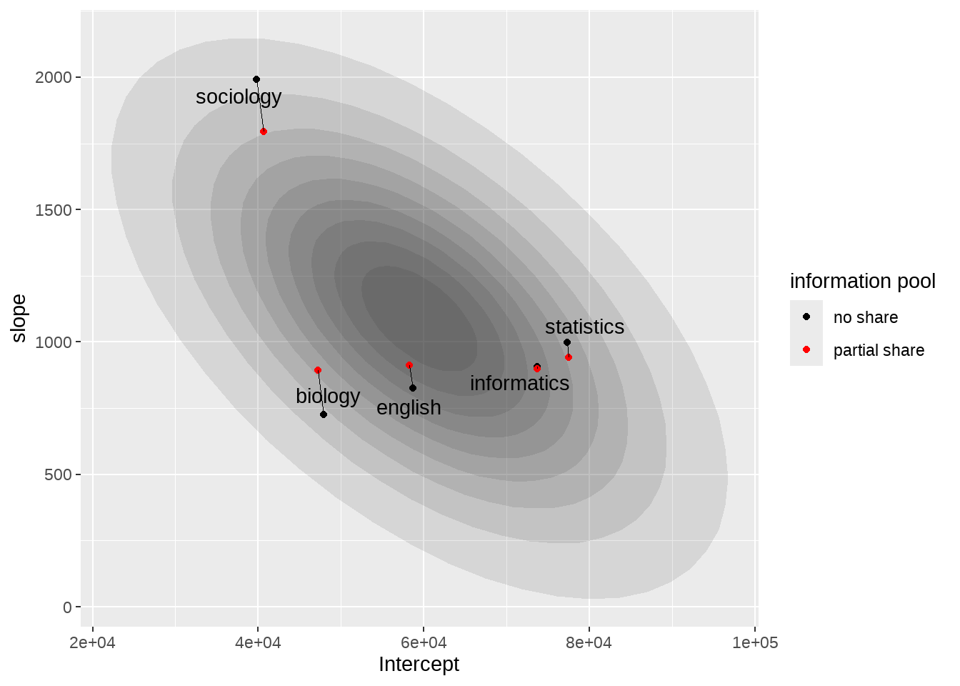
## 5 no_pool statistics 77298. 998.57.7.3 可视化
library(ggrepel)

un_pooling %>%
  dplyr::bind_rows(partial_pooling) %>%
  ggplot(aes(x = Intercept, y = slope)) +
  purrr::map(
    c(seq(from = 0.1, to = 0.9, by = 0.1)),
    .f = function(level) {
      stat_ellipse(
        geom = "polygon", type = "norm",
        size = 0, alpha = 1 / 10, fill = "gray10",
        level = level
      )
    }
  ) +
  geom_point(aes(group = pooled, color = pooled)) +
  geom_line(aes(group = level), size = 1 / 4) +
  # geom_point(data = complete_pooling, size = 4, color = "red") +
  geom_text_repel(
    data = . %>% filter(pooled == "no_pool"),
    aes(label = level)
  ) +
  scale_color_manual(
    name = "information pool",
    values = c(
      "no_pool" = "black",
      "partial_pool" = "red" # ,
      # "complete_pool" = "#A65141"
    ),
    labels = c(
      "no_pool" = "no share",
      "partial_pool" = "partial share" # ,
      # "complete_pool" = "complete share"
    )
  ) #+
# theme_classic()57.8 更多
- 解释模型的含义
lmer(salary ~ 1 + (0 + experience | department), data = df)
# vs
lmer(salary ~ 1 + experience + (0 + experience | department), data = df)
lmer(salary ~ 1 + (1 + experience | department), data = df)## Linear mixed model fit by REML ['lmerMod']
## Formula: salary ~ 1 + (1 + experience | department)
## Data: df
## REML criterion at convergence: 1940.573
## Random effects:
## Groups Name Std.Dev. Corr
## department (Intercept) 24051
## experience 1150 -0.84
## Residual 3527
## Number of obs: 100, groups: department, 5
## Fixed Effects:
## (Intercept)
## 77776
# vs
lmer(salary ~ 1 + (1 | department) + (0 + experience | department), data = df)
## Linear mixed model fit by REML ['lmerMod']
## Formula: salary ~ 1 + (1 | department) + (0 + experience | department)
## Data: df
## REML criterion at convergence: 1941.916
## Random effects:
## Groups Name Std.Dev.
## department (Intercept) 16041
## department.1 experience 1152
## Residual 3526
## Number of obs: 100, groups: department, 5
## Fixed Effects:
## (Intercept)
## 59724- 课后阅读文献,读完后大家一起分享
- 课后阅读 Understanding mixed effects models through data simulation,