第 54 章 统计检验与线性模型的等价性

心理学专业的同学最喜欢的统计方法，估计是方差分析(ANOVA) 和它的堂兄协变量分析 (ANCOVA)，事实上常用的统计检验本质上都是线性模型，所以你学了线性模型，就可以不用学统计检验了，是不是很开心？

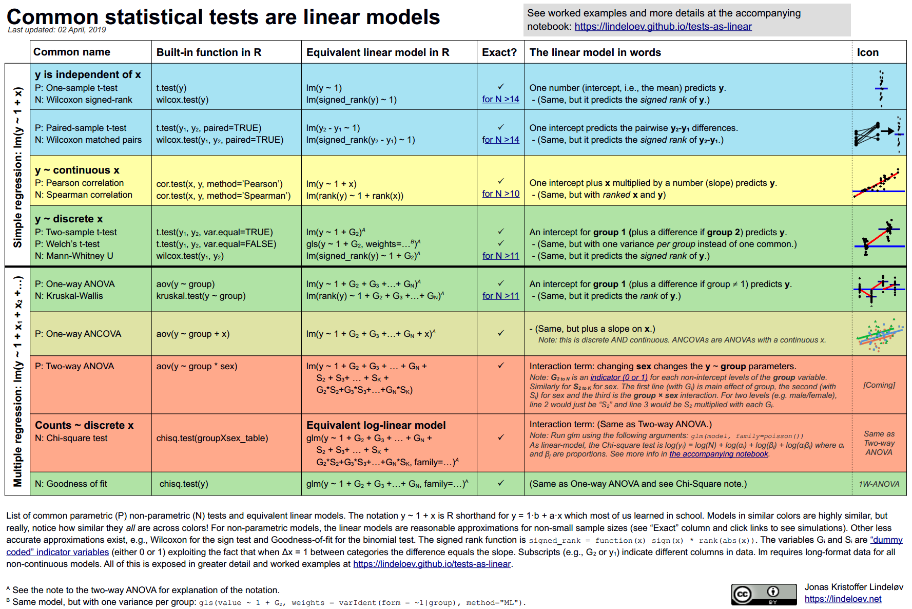
本章，我们将通过几个案例展示统计检验与线性模型的等价性，因此我们这里只关注代码本身，不关注模型的好坏以及模型的解释。部分代码和思想来自 Jonas Kristoffer Lindeløv

experim是一个模拟的数据集，这个虚拟的研究目的是，考察两种不同类型的干预措施对帮助学生应对即将到来的统计学课程的焦虑的影响。实验方案如下：

• 首先，学生完成一定数量的量表(量表1)，包括对统计学课程的害怕(fost)，自信(confid)，抑郁(depress)指标

• 然后，学生被等分成两组，组1 进行技能提升训练；组2进行信心提升训练。训练结束后，完成相同的量表(量表2)

• 三个月后，他们再次完成相同的量表(量表3)

也就说，相同的指标在不同的时期测了三次，目的是考察期间的干预措施对若干指标的影响。

library(tidyverse)

## Warning: package 'ggplot2' was built under R version 4.2.3

## Warning: package 'tibble' was built under R version 4.2.3

## Warning: package 'tidyr' was built under R version 4.2.2

## Warning: package 'readr' was built under R version 4.2.2

## Warning: package 'purrr' was built under R version 4.2.2

## Warning: package 'dplyr' was built under R version 4.2.3

## Warning: package 'stringr' was built under R version 4.2.2

## Warning: package 'lubridate' was built under R version 4.2.2

## ── Attaching core tidyverse packages ──────────────────────── tidyverse 2.0.0 ──
## ✔ dplyr     1.1.2     ✔ readr     2.1.4
## ✔ forcats   1.0.0     ✔ stringr   1.5.0
## ✔ ggplot2   3.4.2     ✔ tibble    3.2.1
## ✔ lubridate 1.9.2     ✔ tidyr     1.3.0
## ✔ purrr     1.0.1     
## ── Conflicts ────────────────────────────────────────── tidyverse_conflicts() ──
## ✖ dplyr::filter() masks stats::filter()
## ✖ dplyr::lag()    masks stats::lag()
## ℹ Use the conflicted package (<http://conflicted.r-lib.org/>) to force all conflicts to become errors

library(knitr)

## Warning: package 'knitr' was built under R version 4.2.3

library(kableExtra)

## 
## Attaching package: 'kableExtra'
## 
## The following object is masked from 'package:dplyr':
## 
##     group_rows

edata <- read_csv("./demo_data/Experim.csv")  %>%
  mutate(group = if_else(group == "maths skills", 1, 2)) %>% 
  mutate(
    across(c(sex, id, group), as.factor)
    )

## Rows: 30 Columns: 18
## ── Column specification ────────────────────────────────────────────────────────
## Delimiter: ","
## chr  (5): sex, group, DepT1gp2, DepT2Gp2, DepT3gp2
## dbl (13): id, age, fost1, confid1, depress1, fost2, confid2, depress2, fost3...
## 
## ℹ Use `spec()` to retrieve the full column specification for this data.
## ℹ Specify the column types or set `show_col_types = FALSE` to quiet this message.

edata

## # A tibble: 30 × 18
##    id    sex     age group fost1 confid1 depress1 fost2 confid2 depress2 fost3
##    <fct> <fct> <dbl> <fct> <dbl>   <dbl>    <dbl> <dbl>   <dbl>    <dbl> <dbl>
##  1 4     male     23 2        50      15       44    48      16       44    45
##  2 10    male     21 2        47      14       42    45      15       42    44
##  3 9     male     25 1        44      12       40    39      18       40    36
##  4 3     male     30 1        47      11       43    42      16       43    41
##  5 12    male     45 2        46      16       44    45      16       45    43
##  6 11    male     22 1        39      13       43    40      20       42    39
##  7 6     male     22 2        32      21       37    33      22       36    32
##  8 5     male     26 1        44      17       46    37      20       47    32
##  9 8     male     23 2        40      22       37    40      23       37    40
## 10 13    male     21 1        47      20       50    45      25       48    46
## # ℹ 20 more rows
## # ℹ 7 more variables: confid3 <dbl>, depress3 <dbl>, exam <dbl>, mah_1 <dbl>,
## #   DepT1gp2 <chr>, DepT2Gp2 <chr>, DepT3gp2 <chr>

glimpse(edata)

## Rows: 30
## Columns: 18
## $ id       <fct> 4, 10, 9, 3, 12, 11, 6, 5, 8, 13, 14, 1, 15, 7, 2, 27, 25, 19…
## $ sex      <fct> male, male, male, male, male, male, male, male, male, male, m…
## $ age      <dbl> 23, 21, 25, 30, 45, 22, 22, 26, 23, 21, 23, 19, 23, 19, 21, 2…
## $ group    <fct> 2, 2, 1, 1, 2, 1, 2, 1, 2, 1, 2, 1, 1, 1, 2, 1, 1, 1, 2, 1, 1…
## $ fost1    <dbl> 50, 47, 44, 47, 46, 39, 32, 44, 40, 47, 38, 32, 39, 36, 37, 4…
## $ confid1  <dbl> 15, 14, 12, 11, 16, 13, 21, 17, 22, 20, 28, 20, 21, 24, 29, 1…
## $ depress1 <dbl> 44, 42, 40, 43, 44, 43, 37, 46, 37, 50, 39, 44, 47, 38, 50, 4…
## $ fost2    <dbl> 48, 45, 39, 42, 45, 40, 33, 37, 40, 45, 37, 28, 35, 32, 36, 4…
## $ confid2  <dbl> 16, 15, 18, 16, 16, 20, 22, 20, 23, 25, 27, 25, 26, 28, 30, 1…
## $ depress2 <dbl> 44, 42, 40, 43, 45, 42, 36, 47, 37, 48, 36, 43, 47, 35, 47, 4…
## $ fost3    <dbl> 45, 44, 36, 41, 43, 39, 32, 32, 40, 46, 32, 23, 35, 30, 34, 3…
## $ confid3  <dbl> 14, 18, 19, 20, 20, 22, 23, 26, 26, 27, 29, 30, 30, 32, 34, 1…
## $ depress3 <dbl> 40, 40, 38, 43, 43, 38, 35, 42, 35, 46, 34, 40, 47, 35, 45, 4…
## $ exam     <dbl> 52, 55, 58, 60, 58, 62, 59, 70, 60, 70, 72, 82, 79, 80, 90, 5…
## $ mah_1    <dbl> 0.5699842, 1.6594031, 3.5404715, 2.4542143, 0.9443036, 1.6257…
## $ DepT1gp2 <chr> "not depressed", "not depressed", "not depressed", "not depre…
## $ DepT2Gp2 <chr> "not depressed", "not depressed", "not depressed", "not depre…
## $ DepT3gp2 <chr> "not depressed", "not depressed", "not depressed", "not depre…

54.1 t检验

首先，我们想检验第一次测量的抑郁得分（depress1）的分布，是否明显偏离正态分布（均值为0），这里的零假设就是正态分布且均值为0； 备选假设就是均值不为0

# Run t-test
model_1_t <- t.test(edata$depress1, mu = 0)
model_1_t

## 
##  One Sample t-test
## 
## data:  edata$depress1
## t = 50.734, df = 29, p-value < 2.2e-16
## alternative hypothesis: true mean is not equal to 0
## 95 percent confidence interval:
##  40.81871 44.24796
## sample estimates:
## mean of x 
##  42.53333

输出结果显示，p-value很小接近0，拒绝零假设，也就说均值不大可能为0。事实上，通过密度图可以看到depress1的分布均值在42附近，与0相距很远。

edata %>%
  ggplot(aes(x = depress1)) +
  geom_density()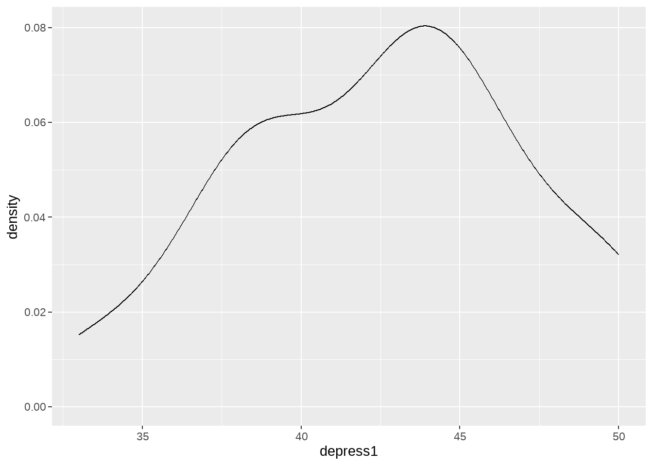

先不管做这个假设有没有意义，我们用线性回归的方法做一遍，

t.test(depress1 ~ 1, data = edata)

## 
##  One Sample t-test
## 
## data:  depress1
## t = 50.734, df = 29, p-value < 2.2e-16
## alternative hypothesis: true mean is not equal to 0
## 95 percent confidence interval:
##  40.81871 44.24796
## sample estimates:
## mean of x 
##  42.53333

# Run equivalent linear model
model_1_lm <- lm(depress1 ~ 1, data = edata)
summary(model_1_lm)

## 
## Call:
## lm(formula = depress1 ~ 1, data = edata)
## 
## Residuals:
##     Min      1Q  Median      3Q     Max 
## -9.5333 -3.5333  0.4667  2.4667  7.4667 
## 
## Coefficients:
##             Estimate Std. Error t value Pr(>|t|)    
## (Intercept)  42.5333     0.8384   50.73   <2e-16 ***
## ---
## Signif. codes:  0 '***' 0.001 '**' 0.01 '*' 0.05 '.' 0.1 ' ' 1
## 
## Residual standard error: 4.592 on 29 degrees of freedom

这个语法lm(y ~ 1)是不是感觉有点点怪怪的呢？左边是响应变量y，右边只有一个1，没有其他预测变量，这里的意思就是用截距预测响应变量y。事实上，也可以看作是检验y变量的均值是否显著偏离0.

为了方便比较两个模型，我们通过broom宏包将两个结果规整在一起，发现两个模型的t-value, estimate 和p.value都是一样的，这与和Jonas Kristoffer Lindeløv表中期望的一样。

library(broom)

## Warning: package 'broom' was built under R version 4.2.3

# tidy() gets model outputs we usually use to report our results
model_1_t_tidy <- tidy(model_1_t) %>% mutate(model = "t.test(y)")
model_1_lm_tidy <- tidy(model_1_lm) %>% mutate(model = "lm(y ~ 1)")

results <- bind_rows(model_1_t_tidy, model_1_lm_tidy) %>%
  select(model, estimate, statistic, p.value)

model	estimate	statistic	p.value
t.test(y)	42.53333	50.73441	0
lm(y ~ 1)	42.53333	50.73441	0

上面例子，我们用不同的方法完成了相同的检验。事实上，在R语言t.test()内部会直接调用lm()函数，其函数语句和我们的这里代码也是一样的。

绝大部分时候，我们想考察实验中的干预是否有效，换句话说，基线得分 depress1 和 干预后得分 depress3 是否存在显著差异？这就需要进行配对样本t检验。

# run paired t-test testing depression from g1 against g2
model_2_t <- t.test(edata$depress1, edata$depress3, paired = TRUE)
model_2_t_tidy <- tidy(model_2_t) %>% mutate(model = "t.test(x, y, paired = TRUE")
model_2_t

## 
##  Paired t-test
## 
## data:  edata$depress1 and edata$depress3
## t = 7.1962, df = 29, p-value = 6.374e-08
## alternative hypothesis: true mean difference is not equal to 0
## 95 percent confidence interval:
##  2.385972 4.280695
## sample estimates:
## mean difference 
##        3.333333

写成线性模型为lm(depress1 - depress3 ~ 1)，即先让两个变量相减，然后去做回归

# run linear model
model_2_lm <- lm(depress1 - depress3 ~ 1, data = edata)
model_2_lm_tidy <- tidy(model_2_lm) %>% mutate(model = "lm(y-x ~ 1)")
summary(model_2_lm)

## 
## Call:
## lm(formula = depress1 - depress3 ~ 1, data = edata)
## 
## Residuals:
##     Min      1Q  Median      3Q     Max 
## -4.3333 -1.3333 -0.3333  1.6667  5.6667 
## 
## Coefficients:
##             Estimate Std. Error t value Pr(>|t|)    
## (Intercept)   3.3333     0.4632   7.196 6.37e-08 ***
## ---
## Signif. codes:  0 '***' 0.001 '**' 0.01 '*' 0.05 '.' 0.1 ' ' 1
## 
## Residual standard error: 2.537 on 29 degrees of freedom

# we combine the two model outputs, rowwise
results <- bind_rows(model_2_t_tidy, model_2_lm_tidy) %>%
  select(model, estimate, statistic, p.value)

model	estimate	statistic	p.value
t.test(x, y, paired = TRUE	3.333333	7.196229	1e-07
lm(y-x ~ 1)	3.333333	7.196229	1e-07

haha，通过这个等价的线性模型，我们似乎可以窥探到配对样本t检验是怎么样工作的。 它depress1 和 depress3一一对应相减后得到新的一列，用新的一列做单样本t检验

# run paired t-test testing depression from g1 against g2
model_2_t2 <- t.test(edata$depress1 - edata$depress3)
model_2_t2_tidy <- tidy(model_2_t2) %>% mutate(model = "t.test(x - y")
model_2_t2

## 
##  One Sample t-test
## 
## data:  edata$depress1 - edata$depress3
## t = 7.1962, df = 29, p-value = 6.374e-08
## alternative hypothesis: true mean is not equal to 0
## 95 percent confidence interval:
##  2.385972 4.280695
## sample estimates:
## mean of x 
##  3.333333

既然是原理这样，那么在回归模型之前，可以在数据框中用depress1 - depress3构建新的一列

# calculate the difference between baseline and tp3 depression
edata <- edata %>%
  mutate(
    dep_slope = depress1 - depress3
  )

model_2_lm2 <- lm(dep_slope ~ 1, data = edata)
model_2_lm2_tidy <- tidy(model_2_lm2) %>% mutate(model = "lm(delta ~ 1)")

最后，把四个模型放在一起

# we combine the three model outputs, rowwise
results <- bind_rows(model_2_t_tidy, model_2_t2_tidy) %>% 
  bind_rows(model_2_lm_tidy) %>%
  bind_rows(model_2_lm2_tidy) %>%
  select(model, estimate, statistic, p.value)

model	estimate	statistic	p.value
t.test(x, y, paired = TRUE	3.333333	7.196229	1e-07
t.test(x - y	3.333333	7.196229	1e-07
lm(y-x ~ 1)	3.333333	7.196229	1e-07
lm(delta ~ 1)	3.333333	7.196229	1e-07

我们看到，四个模型给出了相同的结果。

54.2 关联

两个变量的关联检验，用的也比较常见。比如两个连续型变量，我们可能想知道它们之间的关联，以及这种关联是否显著。

# Run correlation test
model_3_cor <- cor.test(edata$depress3, edata$depress1, method = "pearson")
model_3_cor_tidy <- tidy(model_3_cor) %>% mutate(model = "cor.test(x, y)")
model_3_cor

## 
##  Pearson's product-moment correlation
## 
## data:  edata$depress3 and edata$depress1
## t = 9.2291, df = 28, p-value = 5.486e-10
## alternative hypothesis: true correlation is not equal to 0
## 95 percent confidence interval:
##  0.7378688 0.9354310
## sample estimates:
##       cor 
## 0.8675231

# Run equivalent linear model
model_3_lm <- lm(depress3 ~ depress1, data = edata)
model_3_lm_tidy <- tidy(model_3_lm) %>% mutate(model = "lm(y ~ x)")
summary(model_3_lm)

## 
## Call:
## lm(formula = depress3 ~ depress1, data = edata)
## 
## Residuals:
##     Min      1Q  Median      3Q     Max 
## -5.8421 -1.4744  0.1772  1.2933  4.1966 
## 
## Coefficients:
##             Estimate Std. Error t value Pr(>|t|)    
## (Intercept)  -1.6871     4.4551  -0.379    0.708    
## depress1      0.9613     0.1042   9.229 5.49e-10 ***
## ---
## Signif. codes:  0 '***' 0.001 '**' 0.01 '*' 0.05 '.' 0.1 ' ' 1
## 
## Residual standard error: 2.576 on 28 degrees of freedom
## Multiple R-squared:  0.7526, Adjusted R-squared:  0.7438 
## F-statistic: 85.18 on 1 and 28 DF,  p-value: 5.486e-10

# we combine the two model outputs, rowwise
results <- bind_rows(model_3_cor_tidy, model_3_lm_tidy) %>%
  select(model, term, estimate, statistic, p.value)

model	term	estimate	statistic	p.value
cor.test(x, y)	NA	0.8675231	9.2290506	0.0000000
lm(y ~ x)	(Intercept)	-1.6870911	-0.3786836	0.7077791
lm(y ~ x)	depress1	0.9612952	9.2290506	0.0000000

喔袄，这次的表格有点不一样了。那是因为，线性模型会不仅输出系数，而且还输出了模型的截距，因此两个模型的系数会不一样，但在 t-statistic 和 p.value 是一样的。

54.3 单因素方差分析

我们现在想看看两组（组1=技能提升组；组2=信心提升组）在第一次量表中depress1得分是否有显著区别？

# Run one-way anova
model_4_anova <- aov(depress1 ~ group, data = edata)
model_4_anova_tidy <- tidy(model_4_anova) %>% mutate(model = "aov(y ~ factor(x))")
summary(model_4_anova)

##             Df Sum Sq Mean Sq F value Pr(>F)
## group        1    2.1   2.133   0.098  0.757
## Residuals   28  609.3  21.762

# Run equivalent linear model
model_4_lm <- lm(depress1 ~ group, data = edata)
model_4_lm_tidy <- tidy(model_4_lm) %>% mutate(model = "lm(y ~ factor(x))")
summary(model_4_lm)

## 
## Call:
## lm(formula = depress1 ~ group, data = edata)
## 
## Residuals:
##     Min      1Q  Median      3Q     Max 
## -9.8000 -3.6667  0.4667  2.7333  7.7333 
## 
## Coefficients:
##             Estimate Std. Error t value Pr(>|t|)    
## (Intercept)  42.8000     1.2045  35.534   <2e-16 ***
## group2       -0.5333     1.7034  -0.313    0.757    
## ---
## Signif. codes:  0 '***' 0.001 '**' 0.01 '*' 0.05 '.' 0.1 ' ' 1
## 
## Residual standard error: 4.665 on 28 degrees of freedom
## Multiple R-squared:  0.003489,   Adjusted R-squared:  -0.0321 
## F-statistic: 0.09803 on 1 and 28 DF,  p-value: 0.7565

# we combine the two model outputs, rowwise
results <- bind_rows(model_4_anova_tidy, model_4_lm_tidy) %>%
  select(model, term, estimate, statistic, p.value)

model	term	estimate	statistic	p.value
aov(y ~ factor(x))	group	NA	0.0980306	0.7565262
aov(y ~ factor(x))	Residuals	NA	NA	NA
lm(y ~ factor(x))	(Intercept)	42.8000000	35.5337421	0.0000000
lm(y ~ factor(x))	group2	-0.5333333	-0.3130984	0.7565262

这两个模型输出结果不一样了，且模型的区别似乎有点不好理解。aov评估group变量整体是否有效应， 如果group中的任何一个水平都显著偏离基线水平，那么说明group变量是显著的。

在lm()中，是将group1视为基线, 依次比较其它因子水平（比如group2）与基线group1的之间的偏离，并评估每次这种偏离的显著性；

而aov评估group变量整体是否有效应，即如果group中的任何一个因子水平都显著偏离基线水平，那么说明group变量是显著的。

也就说，aov给出了整体的评估；而lm给出了因子水平之间的评估。

在本案例中，由于group的因子水平只有两个，因此，我们看到两个模型的结论是一致的，p.value = 0.756, 即group分组之间没有显著差异。

同时，我们看到aov没有返回beta系数的估计值，F-value (statistic)值也高于lm线性模型给出的t-statistic。那是因为统计值的计算方法是不一样的造成的，如果 将aov给出F-statustic值的开方，那么就等于lm给出的t-statistic值（限定分组变量只有因子水平时）

# take the square root of the anova stat
sqrt(model_4_anova_tidy$statistic[1])

## [1] 0.3130984

# same as stat from lm
model_4_lm_tidy$statistic[2]

## [1] -0.3130984

# or, square the lm stat
model_4_lm_tidy$statistic[2]^2

## [1] 0.09803063

# same as anova stat
model_4_anova_tidy$statistic[1]

## [1] 0.09803063

54.4 单因素协变量分析

在上面的模型中增加confid1这个指标，考察信心得分是否会影响干预的成功？此时，模型有一个离散变量group，和一个连续变量confid1，这就需要用到协变量分析。

# Run one-way anova
model_5_ancova <- aov(dep_slope ~ group + confid1, data = edata)
model_5_ancova_tidy <- tidy(model_5_ancova) %>% mutate(model = "aov(y ~ x + z)")
summary(model_5_ancova)

##             Df Sum Sq Mean Sq F value Pr(>F)  
## group        1  19.20  19.200   3.134  0.088 .
## confid1      1   2.03   2.032   0.332  0.569  
## Residuals   27 165.43   6.127                 
## ---
## Signif. codes:  0 '***' 0.001 '**' 0.01 '*' 0.05 '.' 0.1 ' ' 1

# Run equivalent linear model
model_5_lm <- lm(dep_slope ~ group + confid1, data = edata)
model_5_lm_tidy <- tidy(model_5_lm) %>% mutate(model = "lm(y ~ x + z)")
summary(model_5_lm)

## 
## Call:
## lm(formula = dep_slope ~ group + confid1, data = edata)
## 
## Residuals:
##     Min      1Q  Median      3Q     Max 
## -4.4851 -2.0413  0.4239  1.5226  4.9094 
## 
## Coefficients:
##             Estimate Std. Error t value Pr(>|t|)  
## (Intercept)  3.46372    1.73752   1.993   0.0564 .
## group2       1.61315    0.90415   1.784   0.0856 .
## confid1     -0.04931    0.08564  -0.576   0.5695  
## ---
## Signif. codes:  0 '***' 0.001 '**' 0.01 '*' 0.05 '.' 0.1 ' ' 1
## 
## Residual standard error: 2.475 on 27 degrees of freedom
## Multiple R-squared:  0.1137, Adjusted R-squared:  0.04809 
## F-statistic: 1.733 on 2 and 27 DF,  p-value: 0.1959

# we combine the two model outputs, rowwise
results <- bind_rows(model_5_ancova_tidy, model_5_lm_tidy) %>%
  select(model, term, estimate, statistic, p.value)

model	term	estimate	statistic	p.value
aov(y ~ x + z)	group	NA	3.1335581	0.0879889
aov(y ~ x + z)	confid1	NA	0.3315903	0.5694932
aov(y ~ x + z)	Residuals	NA	NA	NA
lm(y ~ x + z)	(Intercept)	3.4637195	1.9934809	0.0564018
lm(y ~ x + z)	group2	1.6131503	1.7841656	0.0856403
lm(y ~ x + z)	confid1	-0.0493138	-0.5758388	0.5694932

和单因素方差分析一样，输出结果有一点点不同，但模型输出告诉我们，两个结果是相同的。

aov模型中，group整体的p-value是 ~0.088， lm模型中检验group2偏离group1的p.value是0.086. confidence 这个变量p.value都是0.56993。

唯一不同的地方是aov模型中confidence有一个正的statistic值0.3315 但lm是负的0.5758. 究其原因，可能是它们都很接近0，那么即使数学上很小的差别都会导致结果从0的一边跳到0的另一边。事实上，和单因素方差分析一样，我们将lm模型的confidence的统计值做平方计算，发现与aov的结果是一样样的

# or, square the lm stat
model_5_lm_tidy$statistic[-1]^2

## [1] 3.1832469 0.3315903

# same as anova stat
model_5_ancova_tidy$statistic

## [1] 3.1335581 0.3315903        NA

54.5 双因素方差分析

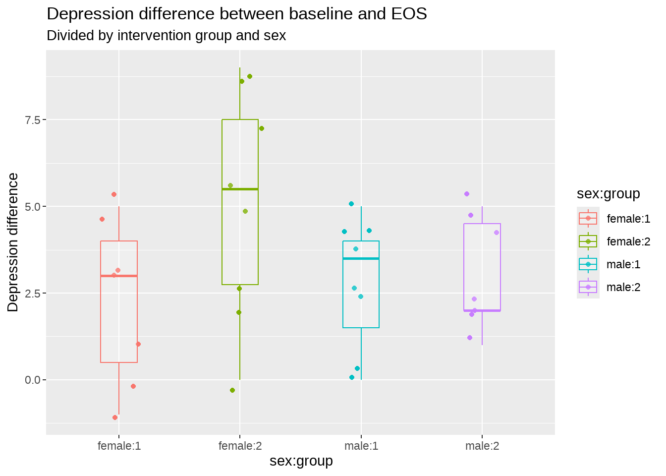
如果我们考察组内性别差异是否会导致depression的变化，那么就需要双因素方差分析，而且两个预测子之间还有相互作用项。

# Run anova
model_6_anova <- aov(dep_slope ~ group * sex, data = edata)
model_6_anova_tidy <- tidy(model_6_anova) %>% mutate(model = "aov(y ~ x * z)")
summary(model_6_anova)

##             Df Sum Sq Mean Sq F value Pr(>F)  
## group        1  19.20  19.200   3.332 0.0794 .
## sex          1   5.15   5.148   0.894 0.3532  
## group:sex    1  12.51  12.515   2.172 0.1525  
## Residuals   26 149.80   5.762                 
## ---
## Signif. codes:  0 '***' 0.001 '**' 0.01 '*' 0.05 '.' 0.1 ' ' 1

# Run equivalent linear model
model_6_lm <- lm(dep_slope ~ group * sex, data = edata)
model_6_lm_tidy <- tidy(model_6_lm) %>% mutate(model = "lm(y ~ x * z)")
summary(model_6_lm)

## 
## Call:
## lm(formula = dep_slope ~ group * sex, data = edata)
## 
## Residuals:
##     Min      1Q  Median      3Q     Max 
## -5.1250 -1.8214  0.4821  1.7187  3.8750 
## 
## Coefficients:
##                Estimate Std. Error t value Pr(>|t|)  
## (Intercept)      2.2857     0.9072   2.519   0.0182 *
## group2           2.8393     1.2423   2.286   0.0307 *
## sexmale          0.4643     1.2423   0.374   0.7116  
## group2:sexmale  -2.5893     1.7569  -1.474   0.1525  
## ---
## Signif. codes:  0 '***' 0.001 '**' 0.01 '*' 0.05 '.' 0.1 ' ' 1
## 
## Residual standard error: 2.4 on 26 degrees of freedom
## Multiple R-squared:  0.1975, Adjusted R-squared:  0.1049 
## F-statistic: 2.133 on 3 and 26 DF,  p-value: 0.1204

# we combine the two model outputs, rowwise
results <- bind_rows(model_6_anova_tidy, model_6_lm_tidy) %>%
  select(model, term, estimate, statistic, p.value)

model	term	estimate	statistic	p.value
aov(y ~ x * z)	group	NA	3.3323638	0.0794378
aov(y ~ x * z)	sex	NA	0.8935272	0.3532257
aov(y ~ x * z)	group:sex	NA	2.1720904	0.1525405
aov(y ~ x * z)	Residuals	NA	NA	NA
lm(y ~ x * z)	(Intercept)	2.2857143	2.5193967	0.0182377
lm(y ~ x * z)	group2	2.8392857	2.2855097	0.0306808
lm(y ~ x * z)	sexmale	0.4642857	0.3737311	0.7116346
lm(y ~ x * z)	group2:sexmale	-2.5892857	-1.4738014	0.1525405

aov()和lm() 公式写法是一样，输出结果又一次不一样，但结论是相同的（尤其是分组变量只有两个水平时候）

aov评估的是 （这些变量作为整体），是否对Y产生差异；而lm 模型，我们评估的是分类变量中的某个因子水平是否与基线水平之间是否有著差异。

最后，为了更好地演示aov与lm之间的等价性，给group弄成一个有多个水平（>2）的因子, 具体过程如下

edata_mock <- edata %>%
  # Add 2 to numeric version of groups
  mutate(group = as.numeric(group) + 2) %>%
  # bind this by row to the origincal eData (with group as numeric)
  bind_rows(edata %>%
    mutate(group = as.numeric(group))) %>%
  # make group a factor again so the correct test is applied
  mutate(group = as.factor(group))

数据没有改，只是复制了一遍，复制出来的数据，因子水平改为3和4， 那么新的数据edata_mock中，group就有四个因子水平（1，2，3，4）

# Run  anova
model_7_anova <- aov(dep_slope ~ group * sex, data = edata_mock)
model_7_anova_tidy <- tidy(model_7_anova) %>% mutate(model = "aov(y ~ x * z)")
summary(model_7_anova)

##             Df Sum Sq Mean Sq F value Pr(>F)  
## group        3  38.40  12.800   2.222 0.0966 .
## sex          1  10.30  10.296   1.787 0.1871  
## group:sex    3  25.03   8.343   1.448 0.2395  
## Residuals   52 299.61   5.762                 
## ---
## Signif. codes:  0 '***' 0.001 '**' 0.01 '*' 0.05 '.' 0.1 ' ' 1

# Run equivalent linear model
model_7_lm <- lm(dep_slope ~ group * sex, data = edata_mock)
model_7_lm_tidy <- tidy(model_7_lm) %>% mutate(model = "lm(y ~ x * z)")
summary(model_7_lm)

## 
## Call:
## lm(formula = dep_slope ~ group * sex, data = edata_mock)
## 
## Residuals:
##     Min      1Q  Median      3Q     Max 
## -5.1250 -2.0000  0.4821  1.8750  3.8750 
## 
## Coefficients:
##                  Estimate Std. Error t value Pr(>|t|)  
## (Intercept)     2.286e+00  9.072e-01   2.519   0.0149 *
## group2          2.839e+00  1.242e+00   2.286   0.0264 *
## group3         -2.809e-15  1.283e+00   0.000   1.0000  
## group4          2.839e+00  1.242e+00   2.286   0.0264 *
## sexmale         4.643e-01  1.242e+00   0.374   0.7101  
## group2:sexmale -2.589e+00  1.757e+00  -1.474   0.1466  
## group3:sexmale  1.689e-15  1.757e+00   0.000   1.0000  
## group4:sexmale -2.589e+00  1.757e+00  -1.474   0.1466  
## ---
## Signif. codes:  0 '***' 0.001 '**' 0.01 '*' 0.05 '.' 0.1 ' ' 1
## 
## Residual standard error: 2.4 on 52 degrees of freedom
## Multiple R-squared:  0.1975, Adjusted R-squared:  0.08945 
## F-statistic: 1.828 on 7 and 52 DF,  p-value: 0.1015

# we combine the two model outputs, rowwise
results <- bind_rows(model_7_anova_tidy, model_7_lm_tidy) %>%
  select(model, term, estimate, statistic, p.value)

model	term	estimate	statistic	p.value
aov(y ~ x * z)	group	NA	2.2215759	0.0966071
aov(y ~ x * z)	sex	NA	1.7870545	0.1871049
aov(y ~ x * z)	group:sex	NA	1.4480603	0.2394867
aov(y ~ x * z)	Residuals	NA	NA	NA
lm(y ~ x * z)	(Intercept)	2.2857143	2.5193967	0.0148675
lm(y ~ x * z)	group2	2.8392857	2.2855097	0.0263899
lm(y ~ x * z)	group3	0.0000000	0.0000000	1.0000000
lm(y ~ x * z)	group4	2.8392857	2.2855097	0.0263899
lm(y ~ x * z)	sexmale	0.4642857	0.3737311	0.7101238
lm(y ~ x * z)	group2:sexmale	-2.5892857	-1.4738014	0.1465634
lm(y ~ x * z)	group3:sexmale	0.0000000	0.0000000	1.0000000
lm(y ~ x * z)	group4:sexmale	-2.5892857	-1.4738014	0.1465634

样本大小翻倍，因此统计值和p-values不一样了。 注意到lm模型，这里现在又两个多余的分组。 因为group3和基线group1完全一样，因此统计为0，p-value 为1；而group 2和group4也是一样的，因此相对基线group1而言，结果是一样的。

所以，相比于做统计检验，我倾向于线性模型，因为lm()除了给出变量作为整体是否对响应变量产生影响外，还提供了更多的因子之间的信息。

edata %>%
  mutate(`sex:group` = interaction(sex, group, sep = ":")) %>%
  ggplot(aes(
    x = sex:group,
    y = dep_slope,
    colour = sex:group
  )) +
  geom_jitter(width = .2) +
  geom_boxplot(width = .3, alpha = .2) +
  labs(
    y = "Depression difference",
    title = "Depression difference between baseline and EOS",
    subtitle = "Divided by intervention group and sex"
  )