第 85 章 探索性数据分析-大学生职业决策
85.1 预备知识
library(tidyverse)

example <-
 tibble::tribble(
   ~name, ~english, ~chinese, ~math, ~sport, ~psy, ~edu,
     "A",     133,    100,    102,     56,    89,   89,
     "B",     120,    120,     86,     88,    45,   75,
     "C",      98,    109,    114,     87,    NA,   84,
     "D",     120,     78,    106,     68,    86,   69,
     "E",     110,     99,    134,     98,    75,   70,
     "F",      NA,    132,    130,     NA,    68,   88
   )

example
## # A tibble: 6 × 7
## name english chinese math sport psy edu
## <chr> <dbl> <dbl> <dbl> <dbl> <dbl> <dbl>
## 1 A 133 100 102 56 89 89
## 2 B 120 120 86 88 45 75
## 3 C 98 109 114 87 NA 84
## 4 D 120 78 106 68 86 69
## 5 E 110 99 134 98 75 70
## 6 F NA 132 130 NA 68 8885.1.1 缺失值检查
我们需要判断每一列的缺失值
example %>%
  summarise(
    na_in_english = sum(is.na(english)),
    na_in_chinese = sum(is.na(chinese)),
    na_in_math    = sum(is.na(math)),
    na_in_sport   = sum(is.na(sport)),
    na_in_psy     = sum(is.na(math)),   # tpyo here
    na_in_edu     = sum(is.na(edu))
  )
## # A tibble: 1 × 6
## na_in_english na_in_chinese na_in_math na_in_sport na_in_psy na_in_edu
## <int> <int> <int> <int> <int> <int>
## 1 1 0 0 1 0 0我们发现,这种写法比较笨,而且容易出错,比如na_in_psy = sum(is.na(math)) 就写错了。那么有没有既偷懒又安全的方法呢?有的。但代价是需要学会across()函数,大家可以在Console中输入?dplyr::across查看帮助文档,或者看第 39 章。
example %>%
  summarise(
    across(everything(), mean)
  )
## # A tibble: 1 × 7
## name english chinese math sport psy edu
## <dbl> <dbl> <dbl> <dbl> <dbl> <dbl> <dbl>
## 1 NA NA 106. 112 NA NA 79.2## # A tibble: 1 × 7
## name english chinese math sport psy edu
## <int> <int> <int> <int> <int> <int> <int>
## 1 0 1 0 0 1 1 085.1.2 数据预处理
- 直接丢弃缺失值所在的行
## # A tibble: 4 × 7
##   name  english chinese  math sport   psy   edu
##   <chr>   <dbl>   <dbl> <dbl> <dbl> <dbl> <dbl>
## 1 A         133     100   102    56    89    89
## 2 B         120     120    86    88    45    75
## 3 D         120      78   106    68    86    69
## 4 E 110 99 134 98 75 70- 用均值代替缺失值
## # A tibble: 6 × 7
##   name  english chinese  math sport   psy   edu
##   <chr>   <dbl>   <dbl> <dbl> <dbl> <dbl> <dbl>
## 1 A        133      100   102  56    89      89
## 2 B        120      120    86  88    45      75
## 3 C         98      109   114  87    72.6    84
## 4 D        120       78   106  68    86      69
## 5 E        110       99   134  98    75      70
## 6 F 116. 132 130 79.4 68 88- 计算总分/均值
## # A tibble: 6 × 8
## # Rowwise:
##   name  english chinese  math sport   psy   edu total
##   <chr>   <dbl>   <dbl> <dbl> <dbl> <dbl> <dbl> <dbl>
## 1 A        133      100   102  56    89      89  569
## 2 B        120      120    86  88    45      75  534
## 3 C         98      109   114  87    72.6    84  565.
## 4 D        120       78   106  68    86      69  527
## 5 E        110       99   134  98    75      70  586
## 6 F 116. 132 130 79.4 68 88 614.## # A tibble: 6 × 8
## # Rowwise:
## name english chinese math sport psy edu mean
## <chr> <dbl> <dbl> <dbl> <dbl> <dbl> <dbl> <dbl>
## 1 A 133 100 102 56 89 89 94.8
## 2 B 120 120 86 88 45 75 89
## 3 C 98 109 114 87 72.6 84 94.1
## 4 D 120 78 106 68 86 69 87.8
## 5 E 110 99 134 98 75 70 97.7
## 6 F 116. 132 130 79.4 68 88 102.- 数据标准化处理
## # A tibble: 6 × 7
## name english chinese math sport psy edu
## <chr> <dbl> <dbl> <dbl> <dbl> <dbl> <dbl>
## 1 A 1.44 -0.339 -0.555 -1.54 1.04 1.10
## 2 B 0.326 0.731 -1.44 0.566 -1.75 -0.464
## 3 C -1.56 0.143 0.111 0.500 0 0.538
## 4 D 0.326 -1.51 -0.333 -0.750 0.852 -1.13
## 5 E -0.531 -0.392 1.22 1.22 0.153 -1.02
## 6 F 0 1.37 0.999 0 -0.292 0.98485.2 开始
85.2.1 文件管理中需要注意的地方
感谢康钦虹同学提供的数据,但这里有几点需要注意的地方:
| 事项 | 问题 | 解决办法 |
|---|---|---|
| 文件名 | excel的文件名是中文 | 用英文,比如 data.xlsx
|
| 列名 | 列名中有-号,大小写不统一 | 规范列名,或用janitor::clean_names()偷懒 |
| 预处理 | 直接在原始数据中新增 | 不要在原始数据上改动,统计工作可以在R里实现 |
| 文件管理 | 没有层级 | 新建data文件夹装数据,与code.Rmd并列 |
data <- readxl::read_excel("demo_data/career-decision.xlsx", skip = 1) %>%
janitor::clean_names()
#glimpse(data)85.2.2 缺失值检查
## # A tibble: 1 × 61
## sex majoy grade from z1 z2 z3 z4 z5 z6 z7 z8 z9
## <int> <int> <int> <int> <int> <int> <int> <int> <int> <int> <int> <int> <int>
## 1 0 0 0 0 0 0 0 0 0 0 0 0 0
## # ℹ 48 more variables: z10 <int>, z11 <int>, z12 <int>, z13 <int>, z14 <int>,
## # z15 <int>, z16 <int>, z17 <int>, z18 <int>, j1 <int>, j2 <int>, j3 <int>,
## # j4 <int>, j5 <int>, j6 <int>, j7 <int>, j8 <int>, j9 <int>, j10 <int>,
## # j11 <int>, j12 <int>, j13 <int>, j14 <int>, j15 <int>, j16 <int>,
## # j17 <int>, j18 <int>, j19 <int>, j20 <int>, j21 <int>, j22 <int>,
## # j23 <int>, j24 <int>, j25 <int>, j26 <int>, j27 <int>, j28 <int>,
## # j29 <int>, j30 <int>, j31 <int>, j32 <int>, j33 <int>, j34 <int>, …没有缺失值,挺好
85.2.3 数据预处理
采用利克特式 5 点计分… (这方面你们懂得比我多)
d <- d %>%
rowwise() %>%
mutate(
environment_exploration = sum(c_across(z1:z5)),
self_exploration = sum(c_across(z6:z9)),
objective_system_exploration = sum(c_across(z10:z15)),
info_quantity_exploration = sum(c_across(z16:z18)),
self_evaluation = sum(c_across(j1:j6)),
information_collection = sum(c_across(j7:j15)),
target_select = sum(c_across(j16:j24)),
formulate = sum(c_across(j25:j32)),
problem_solving = sum(c_across(j33:j39)),
career_exploration = sum(c_across(z1:z18)),
career_decision_making = sum(c_across(j1:j39))
) %>%
select(-starts_with("z"), -starts_with("j")) %>%
ungroup() %>%
mutate(pid = 1:n(), .before = sex) %>%
mutate(
across(c(pid, sex, majoy, grade, from), as_factor)
)
#glimpse(d)85.2.4 标准化
standard <- function(x) {
  (x - mean(x)) / sd(x)
}
d <- d %>%
mutate(
across(where(is.numeric), standard)
)
d## # A tibble: 304 × 16
## pid sex majoy grade from environment_exploration self_exploration
## <fct> <fct> <fct> <fct> <fct> <dbl> <dbl>
## 1 1 1 4 4 2 -1.63 -1.58
## 2 2 1 4 4 1 -1.87 -0.723
## 3 3 2 4 4 2 0.0802 0.132
## 4 4 2 4 4 1 -1.87 -1.15
## 5 5 2 4 4 1 -0.895 -1.58
## 6 6 1 1 4 3 -0.651 1.41
## 7 7 1 4 4 3 -2.36 -0.723
## 8 8 1 4 4 1 -0.407 -1.15
## 9 9 1 4 4 3 -0.651 0.132
## 10 10 1 4 4 2 0.324 0.132
## # ℹ 294 more rows
## # ℹ 9 more variables: objective_system_exploration <dbl>,
## # info_quantity_exploration <dbl>, self_evaluation <dbl>,
## # information_collection <dbl>, target_select <dbl>, formulate <dbl>,
## # problem_solving <dbl>, career_exploration <dbl>,
## # career_decision_making <dbl>85.3 探索
85.3.2 男生女生在职业探索上有所不同?
以性别为例。因为性别变量是男女,仅仅2组,所以检查男女在各自指标上的均值差异,可以用T检验。
## # A tibble: 2 × 12
##   sex   environment_exploration self_exploration objective_system_exploration
##   <fct>                   <dbl>            <dbl>                        <dbl>
## 1 1                      -0.147          -0.0829                       -0.180
## 2 2                       0.165           0.0933                        0.202
## # ℹ 8 more variables: info_quantity_exploration <dbl>, self_evaluation <dbl>,
## #   information_collection <dbl>, target_select <dbl>, formulate <dbl>,
## #   problem_solving <dbl>, career_exploration <dbl>,
## #   career_decision_making <dbl>
你可以给这个图颜色弄得更好看点?
library(ggridges)
d %>%
  ggplot(aes(x = career_exploration, y = sex, fill = sex)) +
  geom_density_ridges()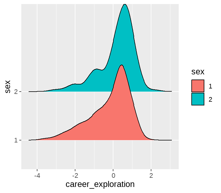
t_test_eq <- t.test(career_exploration ~ sex, data = d, var.equal = TRUE) %>%
  broom::tidy()
t_test_eq
## # A tibble: 1 × 10
## estimate estimate1 estimate2 statistic p.value parameter conf.low conf.high
## <dbl> <dbl> <dbl> <dbl> <dbl> <dbl> <dbl> <dbl>
## 1 -0.367 -0.173 0.194 -3.24 0.00132 302 -0.589 -0.144
## # ℹ 2 more variables: method <chr>, alternative <chr>
t_test_uneq <- t.test(career_exploration ~ sex, data = d, var.equal = FALSE) %>%
  broom::tidy()
t_test_uneq
## # A tibble: 1 × 10
## estimate estimate1 estimate2 statistic p.value parameter conf.low conf.high
## <dbl> <dbl> <dbl> <dbl> <dbl> <dbl> <dbl> <dbl>
## 1 -0.367 -0.173 0.194 -3.27 0.00121 302. -0.588 -0.146
## # ℹ 2 more variables: method <chr>, alternative <chr>当然,也可以用第 56 章介绍的统计推断的方法
library(infer)

obs_diff <- d %>%
  specify(formula = career_exploration ~ sex) %>%
  calculate("diff in means", order = c("1", "2"))
obs_diff
## Response: career_exploration (numeric)
## Explanatory: sex (factor)
## # A tibble: 1 × 1
## stat
## <dbl>
## 1 -0.367
null_dist <- d %>%
  specify(formula = career_exploration ~ sex) %>%
  hypothesize(null = "independence") %>%
  generate(reps = 5000, type = "permute") %>%
  calculate(stat = "diff in means", order = c("1", "2"))
null_dist
## Response: career_exploration (numeric)
## Explanatory: sex (factor)
## Null Hypothesis: independence
## # A tibble: 5,000 × 2
## replicate stat
## <int> <dbl>
## 1 1 -0.0480
## 2 2 -0.164
## 3 3 0.0387
## 4 4 0.224
## 5 5 -0.142
## 6 6 -0.0565
## 7 7 -0.0370
## 8 8 0.0925
## 9 9 0.00575
## 10 10 -0.0370
## # ℹ 4,990 more rows
null_dist %>%
  visualize() +
  shade_p_value(obs_stat = obs_diff, direction = "two_sided")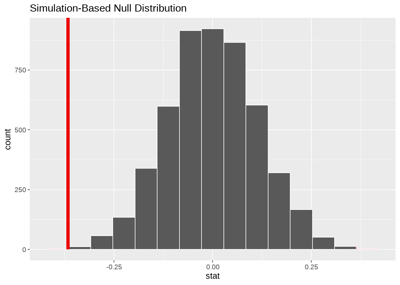
null_dist %>%
  get_p_value(obs_stat = obs_diff, direction = "two_sided") %>%
  #get_p_value(obs_stat = obs_diff, direction = "less") %>%
  mutate(p_value_clean = scales::pvalue(p_value))
## # A tibble: 1 × 2
## p_value p_value_clean
## <dbl> <chr>
## 1 0.0008 <0.001也可以用tidyverse的方法一次性的搞定所有指标
d %>%
  pivot_longer(
    cols = -c(pid, sex, majoy, grade, from),
    names_to = "index",
    values_to = "value"
  ) %>%
  group_by(index) %>%
  summarise(
    broom::tidy( t.test(value ~ sex, data = cur_data()))
  ) %>%
  select(index, estimate, statistic, p.value) %>%
  arrange(p.value)
## # A tibble: 11 × 4
## index estimate statistic p.value
## <chr> <dbl> <dbl> <dbl>
## 1 career_decision_making -0.494 -4.53 0.00000862
## 2 problem_solving -0.470 -4.26 0.0000270
## 3 target_select -0.449 -4.07 0.0000609
## 4 formulate -0.411 -3.72 0.000235
## 5 information_collection -0.411 -3.70 0.000253
## 6 self_evaluation -0.404 -3.65 0.000315
## 7 objective_system_exploration -0.382 -3.40 0.000765
## 8 career_exploration -0.367 -3.27 0.00121
## 9 environment_exploration -0.312 -2.75 0.00629
## 10 info_quantity_exploration -0.274 -2.42 0.0162
## 11 self_exploration -0.176 -1.54 0.12685.3.3 来自不同地方的学生在职业探索上有所不同?
以生源地为例。因为生源地有3类,所以可以使用方差分析。
## # A tibble: 3 × 7
##   term  contrast null.value estimate conf.low conf.high adj.p.value
##   <chr> <chr>         <dbl>    <dbl>    <dbl>     <dbl>       <dbl>
## 1 from  2-1               0   0.382    0.0623     0.701      0.0144
## 2 from  3-1               0   0.287   -0.0386     0.613      0.0964
## 3 from  3-2               0  -0.0943  -0.446      0.257      0.802
library(ggridges)
d %>%
  ggplot(aes(x = career_exploration, y = from, fill = from)) +
  geom_density_ridges()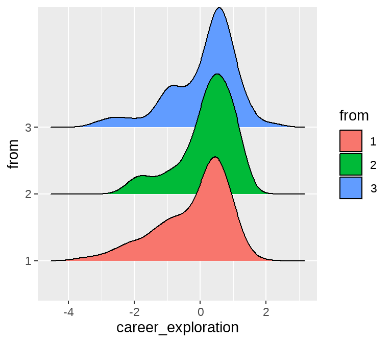
也可以一次性的搞定所有指标
d %>%
  pivot_longer(
    cols = -c(pid, sex, majoy, grade, from),
    names_to = "index",
    values_to = "value"
  ) %>%
  group_by(index) %>%
  summarise(
    broom::tidy( aov(value ~ from, data = cur_data()))
  ) %>%
  select(index, term, statistic, p.value) %>%
  filter(term != "Residuals") %>%
  arrange(p.value)
## # A tibble: 11 × 4
## # Groups: index [11]
## index term statistic p.value
## <chr> <chr> <dbl> <dbl>
## 1 problem_solving from 14.6 0.000000918
## 2 career_decision_making from 14.2 0.00000126
## 3 formulate from 12.2 0.00000781
## 4 information_collection from 10.2 0.0000527
## 5 self_evaluation from 8.91 0.000174
## 6 target_select from 8.45 0.000270
## 7 info_quantity_exploration from 5.78 0.00344
## 8 career_exploration from 4.48 0.0121
## 9 objective_system_exploration from 4.06 0.0181
## 10 environment_exploration from 3.69 0.0260
## 11 self_exploration from 0.699 0.49885.3.4 职业探索和决策之间有关联?
可以用第 51 章线性模型来探索
lm(career_decision_making ~ career_exploration, data = d)##
## Call:
## lm(formula = career_decision_making ~ career_exploration, data = d)
##
## Coefficients:
## (Intercept) career_exploration
## 2.146e-15 7.831e-01不要因为我讲课讲的很垃圾,就错过了R的美,瑕不掩瑜啦。要相信自己,你们是川师研究生中最聪明的。