第 55 章 统计推断

Statistical Inference: A Tidy Approach

55.1 案例1:你会给爱情片还是动作片高分？

这是一个关于电影评分的数据集⁸，

library(tidyverse)
d <- ggplot2movies::movies
d

## # A tibble: 58,788 × 24
##   title     year length budget rating votes    r1    r2
##   <chr>    <int>  <int>  <int>  <dbl> <int> <dbl> <dbl>
## 1 $         1971    121     NA    6.4   348   4.5   4.5
## 2 $1000 a…  1939     71     NA    6      20   0    14.5
## 3 $21 a D…  1941      7     NA    8.2     5   0     0  
## 4 $40,000   1996     70     NA    8.2     6  14.5   0  
## 5 $50,000…  1975     71     NA    3.4    17  24.5   4.5
## 6 $pent     2000     91     NA    4.3    45   4.5   4.5
## # … with 58,782 more rows, and 16 more variables:
## #   r3 <dbl>, r4 <dbl>, r5 <dbl>, r6 <dbl>, r7 <dbl>,
## #   r8 <dbl>, r9 <dbl>, r10 <dbl>, mpaa <chr>,
## #   Action <int>, Animation <int>, Comedy <int>,
## #   Drama <int>, Documentary <int>, Romance <int>,
## #   Short <int>

数据集包含58788 行 和 24 变量

variable	description
title	电影名
year	发行年份
budget	预算金额
length	电影时长
rating	平均得分
votes	投票人数
r1-10	各分段投票人占比
mpaa	MPAA 分级
action	动作片
animation	动画片
comedy	喜剧片
drama	戏剧
documentary	纪录片
romance	爱情片
short	短片

我们想看下爱情片与动作片（不是爱情动作片）的平均得分是否显著不同。

• 首先我们简单的整理下数据，主要是剔除既是爱情片又是动作片的电影

movies_genre_sample <- d %>%
  select(title, year, rating, Action, Romance) %>%
  filter(!(Action == 1 & Romance == 1)) %>% 
  mutate(genre = case_when(
    Action == 1 ~ "Action",
    Romance == 1 ~ "Romance",
    TRUE ~ "Neither"
  )) %>%
  filter(genre != "Neither") %>%
  select(-Action, -Romance) %>%
  group_by(genre) %>%
  #slice_sample(n = 34) %>%  # sample size = 34
  slice_head(n = 34) %>%  
  ungroup()

movies_genre_sample

## # A tibble: 68 × 4
##   title                  year rating genre 
##   <chr>                 <int>  <dbl> <chr> 
## 1 $windle                2002    5.3 Action
## 2 'A' gai waak           1983    7.1 Action
## 3 'A' gai waak juk jaap  1987    7.2 Action
## 4 'Crocodile' Dundee II  1988    5   Action
## 5 'Gator Bait            1974    3.5 Action
## 6 'Sheba, Baby'          1975    5.5 Action
## # … with 62 more rows

• 先看下图形

movies_genre_sample %>%
  ggplot(aes(x = genre, y = rating)) +
  geom_boxplot() +
  geom_jitter()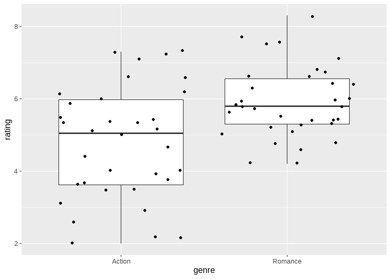

• 看下两种题材电影评分的分布

movies_genre_sample %>%
  ggplot(mapping = aes(x = rating)) +
  geom_histogram(binwidth = 1, color = "white") +
  facet_grid(vars(genre))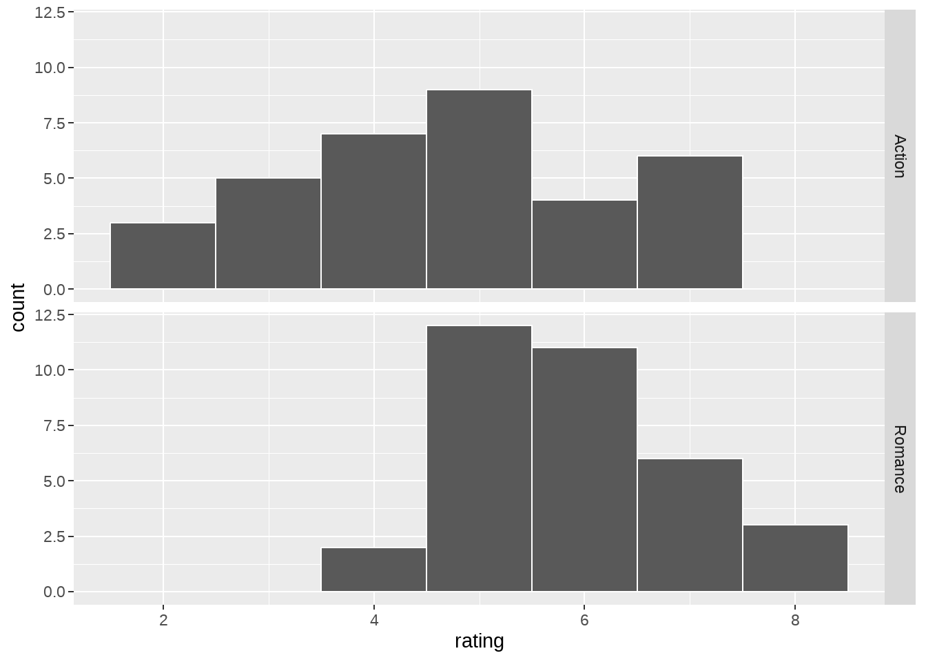

• 统计两种题材电影评分的均值

summary_ratings <- movies_genre_sample %>%
  group_by(genre) %>%
  summarize(
    mean = mean(rating),
    std_dev = sd(rating),
    n = n()
  )
summary_ratings

## # A tibble: 2 × 4
##   genre    mean std_dev     n
##   <chr>   <dbl>   <dbl> <int>
## 1 Action   4.78   1.56     34
## 2 Romance  5.91   0.994    34

55.1.1 传统的基于频率方法的t检验

假设：

• 零假设:

  • \(H_0: \mu_{1} - \mu_{2} = 0\)

• 备选假设:

  • \(H_A: \mu_{1} - \mu_{2} \neq 0\)

两种可能的结论:

• 拒绝 \(H_0\)
• 不能拒绝 \(H_0\)

t_test_eq <- t.test(rating ~ genre,
  data = movies_genre_sample,
  var.equal = TRUE
) %>%
  broom::tidy()
t_test_eq

## # A tibble: 1 × 10
##   estimate estimate1 estimate2 statistic  p.value
##      <dbl>     <dbl>     <dbl>     <dbl>    <dbl>
## 1    -1.12      4.78      5.91     -3.54 0.000736
## # … with 5 more variables: parameter <dbl>,
## #   conf.low <dbl>, conf.high <dbl>, method <chr>,
## #   alternative <chr>

t_test_uneq <- t.test(rating ~ genre,
  data = movies_genre_sample,
  var.equal = FALSE
) %>%
  broom::tidy()
t_test_uneq

## # A tibble: 1 × 10
##   estimate estimate1 estimate2 statistic  p.value
##      <dbl>     <dbl>     <dbl>     <dbl>    <dbl>
## 1    -1.12      4.78      5.91     -3.54 0.000810
## # … with 5 more variables: parameter <dbl>,
## #   conf.low <dbl>, conf.high <dbl>, method <chr>,
## #   alternative <chr>

55.1.2 infer:基于模拟的检验

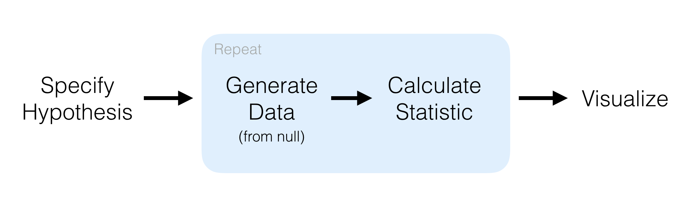
所有的假设检验都符合这个框架⁹:

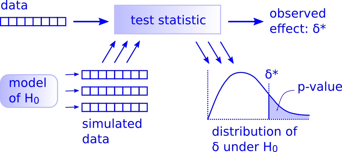
图 55.1: Hypothesis Testing Framework

• 实际观察的差别

library(infer)

obs_diff <- movies_genre_sample %>%
  specify(formula = rating ~ genre) %>%
  calculate(
    stat = "diff in means",
    order = c("Romance", "Action")
  )
obs_diff

## Response: rating (numeric)
## Explanatory: genre (factor)
## # A tibble: 1 × 1
##    stat
##   <dbl>
## 1  1.12

• 模拟

null_dist <- movies_genre_sample %>%
  specify(formula = rating ~ genre) %>%
  hypothesize(null = "independence") %>%
  generate(reps = 5000, type = "permute") %>% 
  calculate(
    stat = "diff in means",
    order = c("Romance", "Action")
  )
head(null_dist)

## Response: rating (numeric)
## Explanatory: genre (factor)
## Null Hypothesis: independence
## # A tibble: 6 × 2
##   replicate    stat
##       <int>   <dbl>
## 1         1  0.0529
## 2         2 -0.447 
## 3         3  0.341 
## 4         4 -0.271 
## 5         5 -0.0941
## 6         6 -0.0706

• 可视化

null_dist %>%
  visualize()

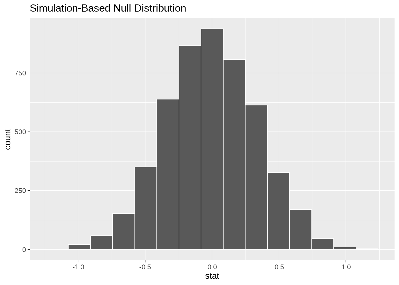
null_dist %>%
  visualize() +
  shade_p_value(obs_stat = obs_diff, direction = "both")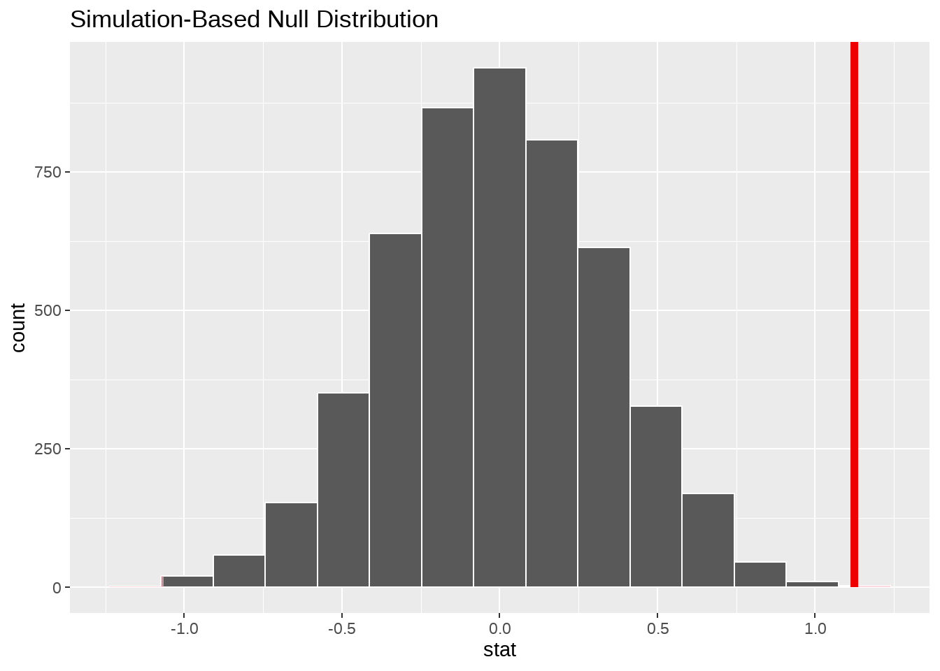

# shade_p_value(bins = 100, obs_stat = obs_diff, direction = "both")

• 计算p值

pvalue <- null_dist %>%
  get_pvalue(obs_stat = obs_diff, direction = "two_sided")

pvalue

## # A tibble: 1 × 1
##   p_value
##     <dbl>
## 1  0.0004

• 结论

在构建的虚拟(\(\Delta = 0\))的平行世界里，出现实际观察值（1.1235）的概率为（4^{-4}）。 如果以(p < 0.05)为标准，我们看到p_value < 0.05, 那我们有足够的证据证明，H0不成立，即爱情电影和动作电影的评分均值存在显著差异，具体来说，动作电影的平均评分要比爱情电影低些。

55.2 案例2: 航天事业的预算有党派门户之见？

美国国家航空航天局的预算是否存在党派门户之见？

gss <- read_rds("./demo_data/gss.rds")

gss %>%
  select(NASA, party) %>%
  count(NASA, party) %>%
  head(8)

## # A tibble: 8 × 3
##   NASA        party     n
##   <fct>       <fct> <int>
## 1 TOO LITTLE  Dem       8
## 2 TOO LITTLE  Ind      13
## 3 TOO LITTLE  Rep       9
## 4 ABOUT RIGHT Dem      22
## 5 ABOUT RIGHT Ind      37
## 6 ABOUT RIGHT Rep      17
## # … with 2 more rows

gss %>%
  ggplot(aes(x = party, fill = NASA)) +
  geom_bar()

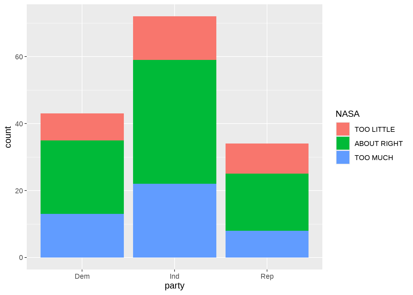
假设：

• 零假设 \(H_0\):

  • 不同党派对预算的态度的构成比(TOO LITTLE, ABOUT RIGHT, TOO MUCH) 没有区别

• 备选假设 \(H_a\):

  • 不同党派对预算的态度的构成比(TOO LITTLE, ABOUT RIGHT, TOO MUCH) 存在区别

两种可能的结论:

• 拒绝 \(H_0\)
• 不能拒绝 \(H_0\)

55.2.1 传统的方法

chisq.test(gss$party, gss$NASA)

## 
##  Pearson's Chi-squared test
## 
## data:  gss$party and gss$NASA
## X-squared = 1.3, df = 4, p-value = 0.9

或者

gss %>%
  chisq_test(NASA ~ party) %>%
  dplyr::select(p_value) %>%
  dplyr::pull()

## [1] 0.8569

55.2.2 infer:Simulation-based tests

obs_stat <- gss %>%
  specify(NASA ~ party) %>%
  calculate(stat = "Chisq")
obs_stat

## Response: NASA (factor)
## Explanatory: party (factor)
## # A tibble: 1 × 1
##    stat
##   <dbl>
## 1  1.33

null_dist <- gss %>%
  specify(NASA ~ party) %>%                     # (1)
  hypothesize(null = "independence") %>%        # (2)
    generate(reps = 5000, type = "permute") %>% # (3)
  calculate(stat = "Chisq")                     # (4)
null_dist

## Response: NASA (factor)
## Explanatory: party (factor)
## Null Hypothesis: independence
## # A tibble: 5,000 × 2
##   replicate  stat
##       <int> <dbl>
## 1         1  1.65
## 2         2  3.52
## 3         3  3.43
## 4         4 11.0 
## 5         5  2.44
## 6         6  8.44
## # … with 4,994 more rows

null_dist %>%
  visualize() +
  shade_p_value(obs_stat = obs_stat, method = "both", direction = "right")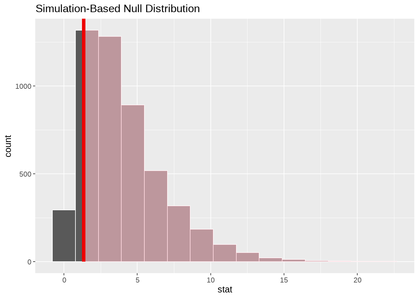

null_dist %>%
  get_pvalue(obs_stat = obs_stat, direction = "greater")

## # A tibble: 1 × 1
##   p_value
##     <dbl>
## 1   0.870

看到 p_value > 0.05，不能拒绝 \(H_0\)，我们没有足够的证据证明党派之间有显著差异

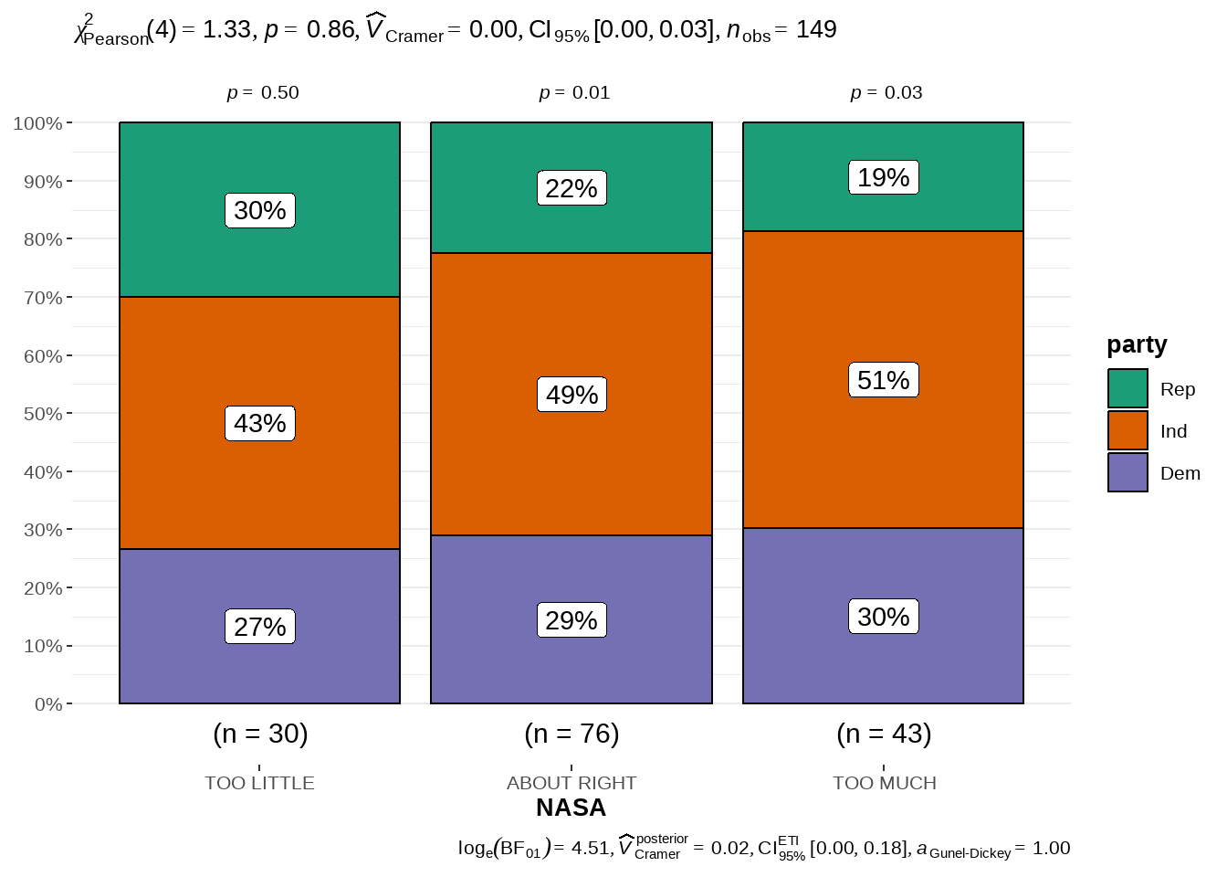
55.2.3 using ggstatsplot::ggbarstats()

library(ggstatsplot)

gss %>% 
  ggbarstats(
    x = party,
    y = NASA
)

55.3 案例3:原住民中的女学生多？

案例 quine 数据集有 146 行 5 列，包含学生的生源、文化、性别和学习成效，具体说明如下

• Eth: 民族背景：原住民与否 (是”A”; 否 “N”)
• Sex: 性别
• Age: 年龄组 (“F0”, “F1,” “F2” or “F3”)
• Lrn: 学习者状态(平均水平 “AL”， 学习缓慢 “SL”)
• Days：一年中缺勤天数

td <- MASS::quine %>%
  as_tibble() %>%
  mutate(
    across(c(Sex, Eth), as_factor)
  )
td

## # A tibble: 146 × 5
##   Eth   Sex   Age   Lrn    Days
##   <fct> <fct> <fct> <fct> <int>
## 1 A     M     F0    SL        2
## 2 A     M     F0    SL       11
## 3 A     M     F0    SL       14
## 4 A     M     F0    AL        5
## 5 A     M     F0    AL        5
## 6 A     M     F0    AL       13
## # … with 140 more rows

从民族背景有两组（A， N）来看，性别为 F 的占比 是否有区别？

td %>% count(Eth, Sex)

## # A tibble: 4 × 3
##   Eth   Sex       n
##   <fct> <fct> <int>
## 1 A     F        38
## 2 A     M        31
## 3 N     F        42
## 4 N     M        35

55.3.1 传统方法

prop.test(table(td$Eth, td$Sex), correct = FALSE)

## 
##  2-sample test for equality of proportions
##  without continuity correction
## 
## data:  table(td$Eth, td$Sex)
## X-squared = 0.0041, df = 1, p-value = 0.9
## alternative hypothesis: two.sided
## 95 percent confidence interval:
##  -0.1564  0.1670
## sample estimates:
## prop 1 prop 2 
## 0.5507 0.5455

55.3.2 基于模拟的方法

被解释变量 sex 中F的占比，解释变量中两组（A，N）

obs_diff <- td %>%
  specify(Sex ~ Eth, success = "F") %>% 
  calculate(
    stat = "diff in props",
    order = c("A", "N")                  
  )

obs_diff

## Response: Sex (factor)
## Explanatory: Eth (factor)
## # A tibble: 1 × 1
##      stat
##     <dbl>
## 1 0.00527

null_distribution <- td %>%
  specify(Sex ~ Eth, success = "F") %>%
  hypothesize(null = "independence") %>%
  generate(reps = 5000, type = "permute") %>%
  calculate(stat = "diff in props", order = c("A", "N"))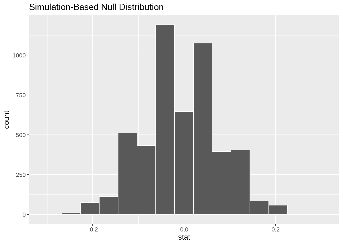

null_distribution %>%
  visualize()

pvalue <- null_distribution %>%
  get_pvalue(obs_stat = obs_diff, direction = "both")

pvalue

## # A tibble: 1 × 1
##   p_value
##     <dbl>
## 1       1

null_distribution %>%
  get_ci(level = 0.95, type = "percentile")

## # A tibble: 1 × 2
##   lower_ci upper_ci
##      <dbl>    <dbl>
## 1   -0.160    0.170

55.4 宏包infer

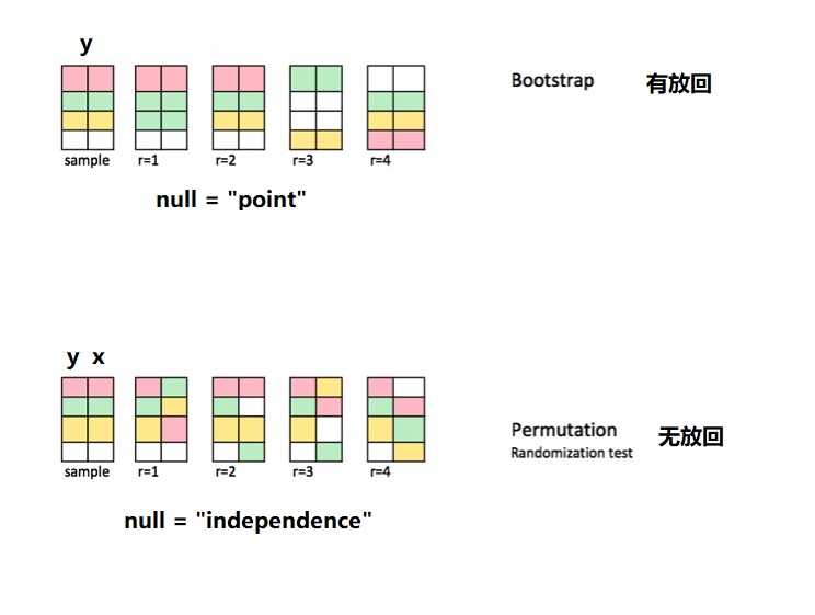
我比较喜欢infer宏包的设计思想，它把统计推断分成了四个步骤

下图可以更好的帮助我们理解infer的工作流程

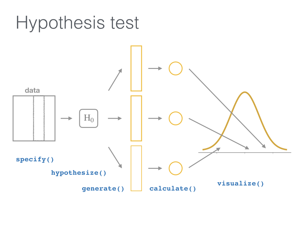
• specify() 指定解释变量和被解释变量 (y ~ x)

• hypothesize() 指定零假设 (比如, independence= y 和 x 彼此独立)

• generate() 从基于零假设的平行世界中抽样:

  • 指定每次重抽样的类型，通俗点讲就是数据洗牌，重抽样type = "bootstrap" (有放回的)，对应的零假设往往是null = “point” ； 重抽样type = "permuting" (无放回的)，对应的零假设往往是null = “independence”, 指的是y和x之间彼此独立的，因此抽样后会重新排列，也就说原先 value1-group1 可能变成了value1-group2，(因为我们假定他们是独立的啊，这种操作，也不会影响y和x的关系)
  • 指定多少组 (reps = 1000)

• calculate() 计算每组(reps)的统计值 (stat = "diff in props")

• visualize() 可视化，对比零假设的分布与实际观察值.

下面是我自己对重抽样的理解

55.5 更多

更多统计推断的内容可参考

• http://infer.netlify.com
• https://moderndive.netlify.com/index.html
• https://moderndive.com/index.html
• https://github.com/tidymodels/infer