第 88 章 探索性数据分析-移民缺口
88.1 引言
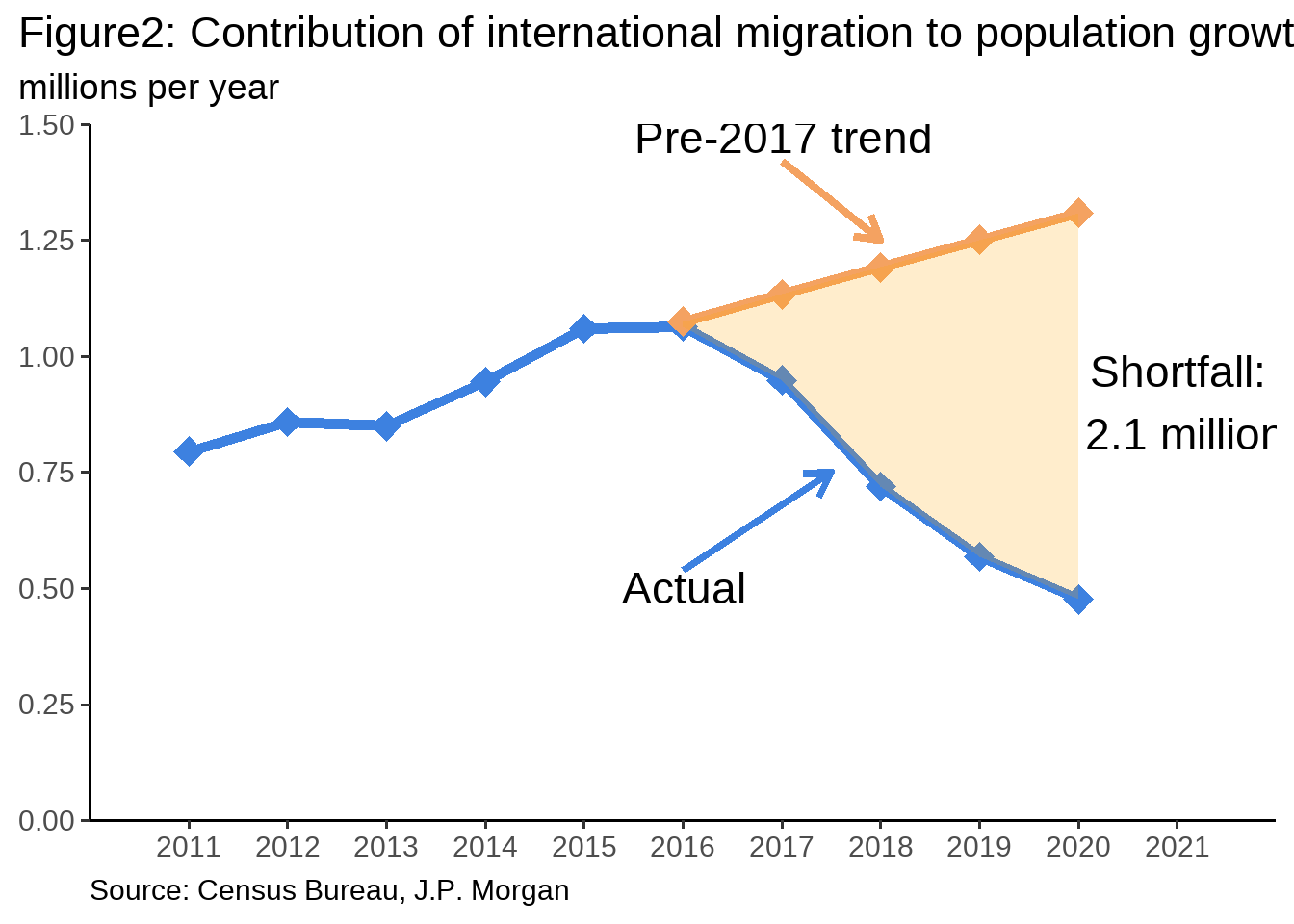
今天看到一张图,觉得很不错,简单清晰。
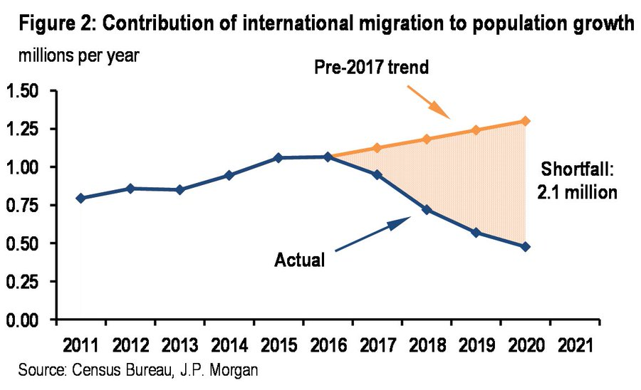
数据是公开的,因此不难找到,我是在这里图中获取。
先观察这张图想表达的意思:
蓝色的是历年移民人口真实数据
依据前6个点(2011年到2016年)建立线性模型,并依此预测后5个点(2016到2021年)的情况,从而得到黄色的直线
预测情况与实际情况的差,得到缺口总数210万
88.2 开始
library(tidyverse)
library(modelr)

df <- tibble::tribble(
  ~year,   ~num,
  2011,  795300,
  2012,  858740,
  2013,  849730,
  2014,  945640,
  2015, 1060000,
  2016, 1065000,
  2017,  948390,
  2018,  719870,
  2019,  568540,
  2020,  477030
) %>%
  mutate(num = num / 1000000)

df
## # A tibble: 10 × 2
## year num
## <dbl> <dbl>
## 1 2011 0.795
## 2 2012 0.859
## 3 2013 0.850
## 4 2014 0.946
## 5 2015 1.06
## 6 2016 1.06
## 7 2017 0.948
## 8 2018 0.720
## 9 2019 0.569
## 10 2020 0.47788.2.2 预测
根据线性模型预测2016年到2020的情况
pred_df <- tibble(
  year = seq(2016, 2020, by = 1)
) %>%
  modelr::add_predictions(model = mod)

pred_df
## # A tibble: 5 × 2
## year pred
## <dbl> <dbl>
## 1 2016 1.08
## 2 2017 1.13
## 3 2018 1.19
## 4 2019 1.25
## 5 2020 1.31合并成新的数据框
## # A tibble: 10 × 3
##     year   num  pred
##    <dbl> <dbl> <dbl>
##  1  2011 0.795 NA
##  2  2012 0.859 NA
##  3  2013 0.850 NA
##  4  2014 0.946 NA
##  5  2015 1.06  NA
##  6  2016 1.06   1.08
##  7  2017 0.948  1.13
##  8  2018 0.720  1.19
##  9  2019 0.569  1.25
## 10  2020 0.477  1.31
# 一个等价的方法
df %>%
  modelr::add_predictions(model = mod) %>%
  mutate(pred = if_else(year < 2016, NA_real_, pred))
88.2.3 可视化
- 基本绘图,画折线图和散点图
combine_df %>%
  ggplot(aes(x = year, y = num)) +
  geom_point() +
  geom_line() +
  geom_line(aes(y = pred)) +
  geom_point(aes(y = pred))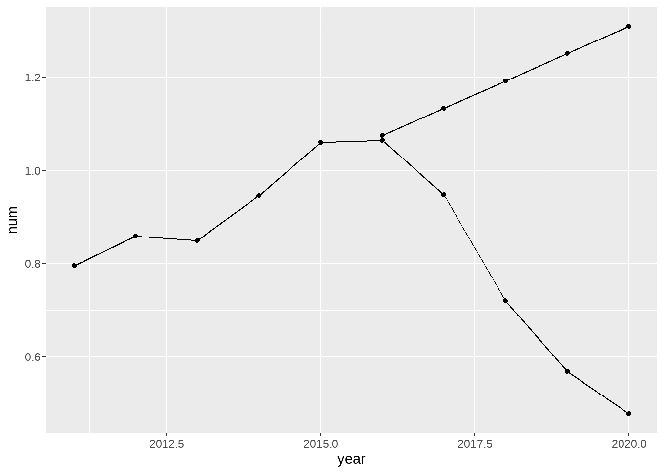
- 调整坐标和配色
combine_df %>%
  ggplot(aes(x = year, y = num)) +
  geom_point(size = 4, fill = "#3D81E0", color = "#3D81E0", shape = 23) +
  geom_line(size = 2, color = "#3D81E0") +
  geom_line(aes(y = pred), size = 2, color = "#f4a261") +
  geom_point(aes(y = pred), size = 4, fill = "#f4a261", color = "#f4a261", shape = 23) +
  labs(
    title = "Figure2: Contribution of international migration to population growth",
    subtitle = "millions per year",
    caption = "Source: Census Bureau, J.P. Morgan",
    x = NULL,
    y = NULL
  ) +
  scale_y_continuous(
    limits = c(0, 1.5),
    breaks = seq(0, 1.5, by = 0.25),
    expand = c(0, 0)
  ) +
  scale_x_continuous(
    limits = c(2011, 2021),
    breaks = seq(2011, 2021, by = 1),
    expand = c(0.1, 0)
  ) +
  theme_classic(base_size = 14) +
  theme(
    legend.position = "none",
    plot.title.position = 'plot',
    plot.caption = element_text(hjust = 0)
  )
- 添加标注
arrows <- tibble::tribble(
  ~x1, ~y1, ~x2, ~y2, ~color,
  2016, 0.54, 2017.5, 0.75, "a",
  2017, 1.42, 2018.0, 1.25, "b"
)


combine_df %>%
  ggplot(aes(x = year, y = num)) +
  geom_point(size = 4, fill = "#3D81E0", color = "#3D81E0", shape = 23) +
  geom_line(size = 2, color = "#3D81E0") +
  geom_line(aes(y = pred), size = 2, color = "#f4a261") +
  geom_point(aes(y = pred), size = 4, fill = "#f4a261", color = "#f4a261", shape = 23) +
  geom_ribbon(
    aes(ymin = num, ymax = pred),
    fill = "orange",
    alpha = 0.2
  ) +
  geom_segment(
    data = arrows,
    aes(x = x1, y = y1, xend = x2, yend = y2, color = color),
    arrow = arrow(length = unit(0.15, "inch")), size = 1.5
  ) +
  annotate("text",
    x = c(2017, 2016, 2021), y = c(1.47, 0.5, 0.9),
    size = 6, face = "bold",
    label = c("Pre-2017 trend", "Actual", "Shortfall:\n 2.1 million")
  ) +
  labs(
    title = "Figure2: Contribution of international migration to population growth",
    subtitle = "millions per year",
    caption = "Source: Census Bureau, J.P. Morgan",
    x = NULL,
    y = NULL
  ) +
  scale_y_continuous(
    limits = c(0, 1.5),
    breaks = seq(0, 1.5, by = 0.25),
    expand = c(0, 0)
  ) +
  scale_x_continuous(
    limits = c(2011, 2021),
    breaks = seq(2011, 2021, by = 1),
    expand = c(0.1, 0)
  ) +
  scale_color_manual(
    values = c(a = "#3D81E0", b = "#f4a261")
  ) +
  theme_classic(base_size = 14) +
  theme(
    legend.position = "none",
    plot.title.position = 'plot',
    plot.caption = element_text(hjust = 0)
  )
- 保存
ggsave("migration.pdf", width = 8, height = 5)