第 12 章数据处理

我们用一个应用场景，复习上两章讲的数据类型和数据结构等概念。比如，这里有一个表格

如果构建学生们的成绩，需要用到是向量，一列就可以了。
如果构建学生的各科成绩，需要用到是矩阵，因为此时需要多列，不同的列对应不同的科目。
如果构建学生综合信息（性别，年龄，各科成绩，是否喜欢R），需要用到的是列表，因为除了各科成绩列，还需要其它数据类型的列。
当然，构建学生综合信息的表格，最好还是用数据框，因为这些信息是等长的，而且符合人的理解习惯, 所以，我们会经常和数据框打交道。

数据框的特性很丰富，在于：

第一，它是列表的特殊形式，可以存储不同类型的数据。
第二，它要求每个元素长度必须一致，因此长的像矩阵。
第三，它的每个元素就是一个是向量，而R语言有个优良特性，就是向量化操作，因此，使用函数非常方便。

本章我们介绍tidyverse里被誉为“瑞士军刀”的数据处理的工具dplyr宏包。首先，我们加载该宏包

library(dplyr)

dplyr 定义了数据处理的规范语法，其中主要包含以下10个主要的函数。

mutate(), select(), rename() , filter()
summarise(), group_by(), arrange()
left_join(), right_join()， full_join()

我们用一个案例依次讲解这些函数的功能。假定这里有三位同学的英语和数学成绩

df <- readr::read_csv(here::here("demo_data", "score.csv"))
df

## # A tibble: 6 × 3
##   name  type    score
##   <chr> <chr>   <dbl>
## 1 Alice english    80
## 2 Alice math       60
## 3 Bob   english    70
## 4 Bob   math       69
## 5 Carol english    80
## 6 Carol math       90

12.1 新增一列 `mutate()`

同学们表现不错，分别得到额外的奖励分 c(2, 5, 9, 8, 5, 6)

reward <- c(2, 5, 9, 8, 5, 6)

那么，如何把奖励分加到表中呢？用mutate()函数可以这样写第一次觉得这个单词很陌生，可以理解为modify

mutate(.data = df, extra = reward)

## # A tibble: 6 × 4
##   name  type    score extra
##   <chr> <chr>   <dbl> <dbl>
## 1 Alice english    80     2
## 2 Alice math       60     5
## 3 Bob   english    70     9
## 4 Bob   math       69     8
## 5 Carol english    80     5
## 6 Carol math       90     6

mutate()函数的功能是给数据框新增一列，使用语法为 mutate(.data = df, name = value)：

第一个参数.data，接受要处理的数据框，比如这里的df。
第二个参数是Name-value对, 比如extra = reward，
- 等号左边，是我们为新增的一列取的名字，比如这里的extra，因为数据框每一列都是要有名字的；
- 等号右边，是打算并入数据框的向量，比如这里的reward，它是装着学生成绩的向量。注意，向量的长度，
  - 要么与数据框的行数等长，比如这里向量长度为6；
  - 要么长度为1，即，新增的这一列所有的值都是一样的(循环补齐机制)。

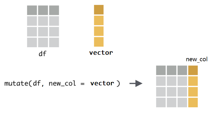
因为mutate()函数处理的是数据框，并且固定放置在第一位置上（几乎所有dplyr的函数都是这样要求的），所以这个.data可以偷懒不写，直接写mutate(df, extra = reward)。另外，如果想同时新增多个列，只需要提供多个Name-value对即可，比如

mutate(df, 
       extra1 = c(2, 5, 9, 8, 5, 6),
       extra2 = c(1, 2, 3, 3, 2, 1),
       extra3 = c(8)
       )

12.2 管道 `%>%`

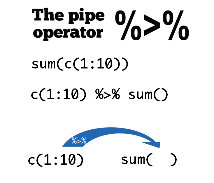
实际运用中，我们经常要使用函数，比如计算向量c(1:10)所有元素值的和

sum(c(1:10))

## [1] 55

现在有个与上面的等价的写法，就是使用管道操作符%>%。

c(1:10) %>% sum()

## [1] 55

这条语句的意思是f(x) 写成 x %>% f()，这里向量 c(1:10) 通过管道操作符 %>% ，传递到函数sum()的第一个参数位置，即sum(c(1:10))，这个 %>% 管道操作符还是很形象的。在Windows系统中可以通过Ctrl + Shift + M 快捷键产生 %>%，苹果系统对应的快捷键是Cmd + Shift + M。

通过下图图示可以看到管道操作符就像生产线上的传送带一样，将数据运入函数中。

当执行多个函数操作的时候，管道操作符 %>% 就显得格外方便，代码可读性也更强。比如

sqrt(sum(abs(c(-10:10))))

## [1] 10.48809

使用管道操作符

c(-10:10) %>% abs() %>% sum() %>% sqrt()

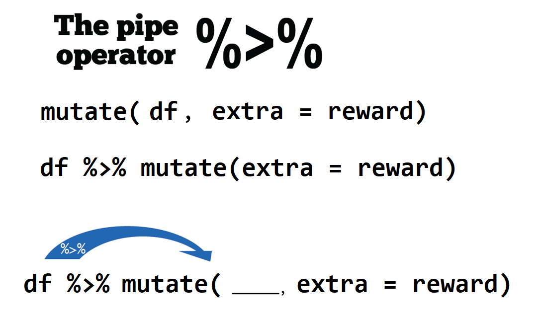
## [1] 10.48809

那么，之前增加学生奖励分成绩的语句 mutate(df, extra = reward)，也可以使用管道

# using `%>%`
df %>% mutate(extra = reward)

## # A tibble: 6 × 4
##   name  type    score extra
##   <chr> <chr>   <dbl> <dbl>
## 1 Alice english    80     2
## 2 Alice math       60     5
## 3 Bob   english    70     9
## 4 Bob   math       69     8
## 5 Carol english    80     5
## 6 Carol math       90     6

是不是很赞⁴。

12.3 向量函数与mutate()

mutate()函数的本质还是第 6 章介绍向量函数和向量化操作，只不过是换作在数据框中完成，这样更能形成“据框进、数据框出”的思维，方便快捷地构思并统计任务⁵。

比如，我们想计算每位同学分数的平方，然后构建数据框新的一列，我们可以用第 7 章函数的方法，自定义calc_square()函数

calc_square <- function(x) {
  x^2
}

df %>% 
  mutate(new_col = calc_square(score))

## # A tibble: 6 × 4
##   name  type    score new_col
##   <chr> <chr>   <dbl>   <dbl>
## 1 Alice english    80    6400
## 2 Alice math       60    3600
## 3 Bob   english    70    4900
## 4 Bob   math       69    4761
## 5 Carol english    80    6400
## 6 Carol math       90    8100

在mutate()中引用数据框的某一列名，实际上是引用了列名对应的整个向量, 所以，这里我们传递score到calc_square()，就是把整个score向量传递给calc_square().

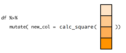
几何算符（这里是平方）是向量化的，因此calc_square()会对输入的score向量，返回一个等长的向量。

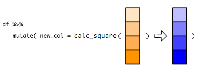
mutate() 拿到这个新的向量后，就在原有数据框中添加新的一列new_col

12.4 保存为新的数据框

现在有个问题，此时 df 有没发生变化？是否包含额外的奖励分呢？事实上，此时df并没有发生改变，还是原来的状态。如果需要保存计算结果，就需要把计算的结果重新赋值给新的对象，当然，也可以赋值给df本身，这样df存储的数据就更新为计算后的结果。

好，现在我们把添加奖励分、计算总成绩和保存结果这三个步骤一气呵成的完成

df_new <- df %>% 
  mutate(extra = reward) %>% 
  mutate(total = score + extra)

df_new

## # A tibble: 6 × 5
##   name  type    score extra total
##   <chr> <chr>   <dbl> <dbl> <dbl>
## 1 Alice english    80     2    82
## 2 Alice math       60     5    65
## 3 Bob   english    70     9    79
## 4 Bob   math       69     8    77
## 5 Carol english    80     5    85
## 6 Carol math       90     6    96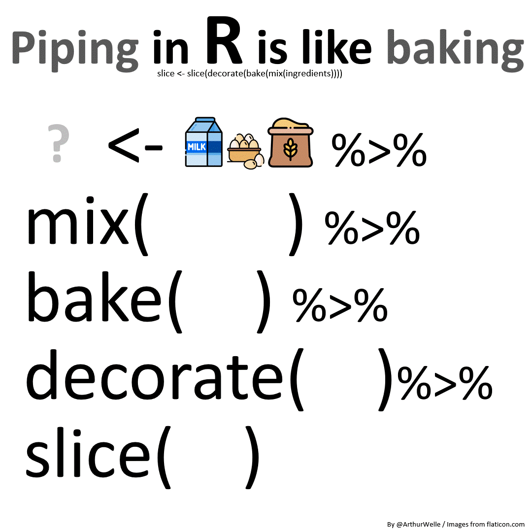

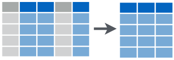
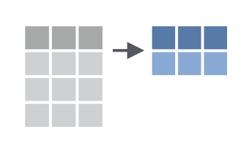
12.5 选取列 `select()`

select()顾名思义选择，就是选择数据框的某一列，或者某几列。

我们以上面学生成绩的数据框为例，这里选择name列

df_new %>% select(name)

## # A tibble: 6 × 1
##   name 
##   <chr>
## 1 Alice
## 2 Alice
## 3 Bob  
## 4 Bob  
## 5 Carol
## 6 Carol

注意，结果是只有一列的数据框（仍然数据框喔，数据框进数据框出是dplyr函数的第二个特点）。如果要选取多列，就再多写几个列名就行了

df_new %>% select(name, extra)

## # A tibble: 6 × 2
##   name  extra
##   <chr> <dbl>
## 1 Alice     2
## 2 Alice     5
## 3 Bob       9
## 4 Bob       8
## 5 Carol     5
## 6 Carol     6

df_new %>% select(name, score, extra, total)

## # A tibble: 6 × 4
##   name  score extra total
##   <chr> <dbl> <dbl> <dbl>
## 1 Alice    80     2    82
## 2 Alice    60     5    65
## 3 Bob      70     9    79
## 4 Bob      69     8    77
## 5 Carol    80     5    85
## 6 Carol    90     6    96

如果不想要某列，可以在变量前面加 - 或者 !，两者的结果是一样的。

df_new %>% select(-type)

## # A tibble: 6 × 4
##   name  score extra total
##   <chr> <dbl> <dbl> <dbl>
## 1 Alice    80     2    82
## 2 Alice    60     5    65
## 3 Bob      70     9    79
## 4 Bob      69     8    77
## 5 Carol    80     5    85
## 6 Carol    90     6    96

df_new %>% select(!type)

## # A tibble: 6 × 4
##   name  score extra total
##   <chr> <dbl> <dbl> <dbl>
## 1 Alice    80     2    82
## 2 Alice    60     5    65
## 3 Bob      70     9    79
## 4 Bob      69     8    77
## 5 Carol    80     5    85
## 6 Carol    90     6    96

也可以通过位置索引进行选取，比如选取头三列

df_new %>% select(1, 2, 3)

## # A tibble: 6 × 3
##   name  type    score
##   <chr> <chr>   <dbl>
## 1 Alice english    80
## 2 Alice math       60
## 3 Bob   english    70
## 4 Bob   math       69
## 5 Carol english    80
## 6 Carol math       90

df_new %>% select(2:3)

## # A tibble: 6 × 2
##   type    score
##   <chr>   <dbl>
## 1 english    80
## 2 math       60
## 3 english    70
## 4 math       69
## 5 english    80
## 6 math       90

如果要选取数据框的列很多，我们也可以先观察列名的特征，用特定的函数进行选取，比如选取以”s”开头的列

df_new %>% select(starts_with("s"))

## # A tibble: 6 × 1
##   score
##   <dbl>
## 1    80
## 2    60
## 3    70
## 4    69
## 5    80
## 6    90

选取以”e”结尾的列

df_new %>% select(ends_with("e"))

## # A tibble: 6 × 3
##   name  type    score
##   <chr> <chr>   <dbl>
## 1 Alice english    80
## 2 Alice math       60
## 3 Bob   english    70
## 4 Bob   math       69
## 5 Carol english    80
## 6 Carol math       90

选取含有以”score”的列

df_new %>% select(contains("score"))

## # A tibble: 6 × 1
##   score
##   <dbl>
## 1    80
## 2    60
## 3    70
## 4    69
## 5    80
## 6    90

当然，也可以通过变量的类型来选取，比如选取所有字符串类型的列

df_new %>% select(where(is.character))

## # A tibble: 6 × 2
##   name  type   
##   <chr> <chr>  
## 1 Alice english
## 2 Alice math   
## 3 Bob   english
## 4 Bob   math   
## 5 Carol english
## 6 Carol math

选取所有数值类型的列

df_new %>% select(where(is.numeric))

## # A tibble: 6 × 3
##   score extra total
##   <dbl> <dbl> <dbl>
## 1    80     2    82
## 2    60     5    65
## 3    70     9    79
## 4    69     8    77
## 5    80     5    85
## 6    90     6    96

选取所有数值类型的并且以”s”开头的列

df_new %>% select(where(is.numeric) & starts_with("t"))

## # A tibble: 6 × 1
##   total
##   <dbl>
## 1    82
## 2    65
## 3    79
## 4    77
## 5    85
## 6    96

选取以”s”开头或者以”e”结尾的列

df_new %>% select(starts_with("s") | ends_with("e"))

## # A tibble: 6 × 3
##   score name  type   
##   <dbl> <chr> <chr>  
## 1    80 Alice english
## 2    60 Alice math   
## 3    70 Bob   english
## 4    69 Bob   math   
## 5    80 Carol english
## 6    90 Carol math

df_new %>% select(!starts_with("s"))

## # A tibble: 6 × 4
##   name  type    extra total
##   <chr> <chr>   <dbl> <dbl>
## 1 Alice english     2    82
## 2 Alice math        5    65
## 3 Bob   english     9    79
## 4 Bob   math        8    77
## 5 Carol english     5    85
## 6 Carol math        6    96

12.6 修改列名 `rename()`

用rename()修改列的名字, 具体方法是rename(.data, new_name = old_name)，和mutate()一样，等号左边是新的变量名，右边是已经存在的变量名（这是dplyr函数的第三个特征⁶）。比如，我们这里将total修改为total_score

df_new %>% 
  select(name, type, total) %>% 
  rename(total_score = total)

## # A tibble: 6 × 3
##   name  type    total_score
##   <chr> <chr>         <dbl>
## 1 Alice english          82
## 2 Alice math             65
## 3 Bob   english          79
## 4 Bob   math             77
## 5 Carol english          85
## 6 Carol math             96

12.7 筛选 `filter()`

前面select()是列方向的选择，而用filter()函数，我们可以对数据框行方向进行筛选，选出符合特定条件的某些行。

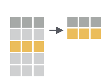
注意，这里filter()函数不是字面上“过滤掉”的意思，而是保留符合条件的行，也就说keep，不是drop的意思。第一次会有一点点迷惑，我相信习惯就好了。

比如这里把成绩等于90分的同学筛选出来。

df_new %>% filter(score = 90)

## Error in `filter()`:
## ! We detected a named input.
## ℹ This usually means that you've used `=` instead of `==`.
## ℹ Did you mean `score == 90`?

注意，这里判断是否相等要使用 == 而不是 =

df_new %>% filter(score == 90)

## # A tibble: 1 × 5
##   name  type  score extra total
##   <chr> <chr> <dbl> <dbl> <dbl>
## 1 Carol math     90     6    96

R提供了其他比较关系的算符: <, >, <=, >=, == (equal), != (not equal), %in%, is.na() 和 !is.na() .

比如把成绩大于等于80分的同学筛选出来

df_new %>% filter(score >= 80)

## # A tibble: 3 × 5
##   name  type    score extra total
##   <chr> <chr>   <dbl> <dbl> <dbl>
## 1 Alice english    80     2    82
## 2 Carol english    80     5    85
## 3 Carol math       90     6    96

也可以限定多个条件进行筛选, 比如，限定英语学科，同时要求成绩高于75分的所有条目筛选出来

df_new %>% filter(type == "english", score >= 75)

## # A tibble: 2 × 5
##   name  type    score extra total
##   <chr> <chr>   <dbl> <dbl> <dbl>
## 1 Alice english    80     2    82
## 2 Carol english    80     5    85

也就说，逗号分隔的两个条件都要满足。

12.7.1 常见的错误

filter()函数两个常见的错误:

把 “=” 误认为 “==”

df_new %>% filter(type = "english")   # error
df_new %>% filter(type == "english")

忘记引号

df_new %>% filter(type == english)   # error
df_new %>% filter(type == "english")

12.7.2 逻辑算符

多个参数的情形，本质上是逻辑与的关系，每个条件都返回TRUE

df_new %>% filter(type == "english" & score >= 75)

## # A tibble: 2 × 5
##   name  type    score extra total
##   <chr> <chr>   <dbl> <dbl> <dbl>
## 1 Alice english    80     2    82
## 2 Carol english    80     5    85

当然也可以使用其他的布尔算符 (& is “and,” | is “or,” and ! is “not.”).

比如，以下代码找出成绩等于70或者等于90的行

df_new %>% filter(score == 70 | score == 90)

## # A tibble: 2 × 5
##   name  type    score extra total
##   <chr> <chr>   <dbl> <dbl> <dbl>
## 1 Bob   english    70     9    79
## 2 Carol math       90     6    96

在filter()中有一个非常有效的等价方法，即使用 x %in% y，意思是如果当前x的值是向量y的一员，那么就选出当前行，因此，我们可以重写上面代码:

df_new %>% filter(score %in% c(70, 90))

## # A tibble: 2 × 5
##   name  type    score extra total
##   <chr> <chr>   <dbl> <dbl> <dbl>
## 1 Bob   english    70     9    79
## 2 Carol math       90     6    96

当然还可以配合一些函数使用，比如把最高分的同学找出来

df_new %>% filter(score == max(score))

## # A tibble: 1 × 5
##   name  type  score extra total
##   <chr> <chr> <dbl> <dbl> <dbl>
## 1 Carol math     90     6    96

把成绩高于均值的找出来

df_new %>% filter(score > mean(score))

## # A tibble: 3 × 5
##   name  type    score extra total
##   <chr> <chr>   <dbl> <dbl> <dbl>
## 1 Alice english    80     2    82
## 2 Carol english    80     5    85
## 3 Carol math       90     6    96

12.8 统计汇总 `summarise()`

summarise()函数非常强大，主要用于统计汇总，往往与其他函数配合使用，比如计算所有同学考试成绩的均值

df_new %>% summarise(mean_score = mean(score))

## # A tibble: 1 × 1
##   mean_score
##        <dbl>
## 1       74.8

计算所有同学的考试成绩的标准差

df_new %>% summarise( sd_score = sd(score))

## # A tibble: 1 × 1
##   sd_score
##      <dbl>
## 1     10.6

还可以同时完成多个统计

df_new %>% summarise(
  mean_score   = mean(score),
  median_score = median(score),
  n            = n(),
  sum          = sum(score)
)

## # A tibble: 1 × 4
##   mean_score median_score     n   sum
##        <dbl>        <dbl> <int> <dbl>
## 1       74.8           75     6   449

summarise() 与 mutate() 一样，也是创建新的变量（新的一列），仍然遵循等号左边是新的列名，等号右边是基于原变量的统计。区别在于，mutate()是在原数据框的基础上增加新的一列；而summarise()在成立的新的数据框中创建一列。

12.9 分组统计 `group_by()`

实际运用中，summarise()函数往往配合group_by()一起使用，即，先分组再统计。

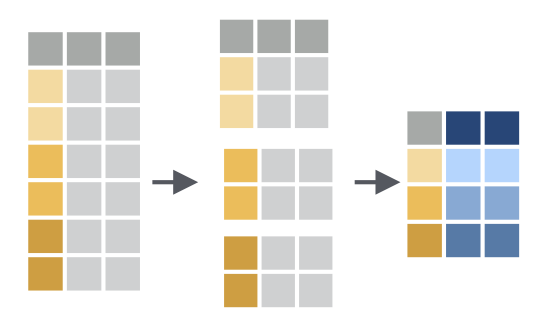
比如，我们想统计每个学生的平均成绩，那么就需要先按照学生name分组，然后每组求平均

df_new %>%
  group_by(name) %>%
  summarise(
    mean_score = mean(total),
    sd_score   = sd(total)
  )

## # A tibble: 3 × 3
##   name  mean_score sd_score
##   <chr>      <dbl>    <dbl>
## 1 Alice       73.5    12.0 
## 2 Bob         78       1.41
## 3 Carol       90.5     7.78

12.10 排序 `arrange()`

arrange()这个很好理解的，就是按照某个变量排序。

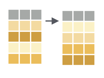
比如我们按照考试总成绩从低到高排序，然后输出

df_new %>% arrange(total)

## # A tibble: 6 × 5
##   name  type    score extra total
##   <chr> <chr>   <dbl> <dbl> <dbl>
## 1 Alice math       60     5    65
## 2 Bob   math       69     8    77
## 3 Bob   english    70     9    79
## 4 Alice english    80     2    82
## 5 Carol english    80     5    85
## 6 Carol math       90     6    96

默认情况是从小到大排序，如果从高到低降序排序呢，有两种方法，第一种方法是在用于排序的变量前面加 - 号，

df_new %>% arrange(-total)

## # A tibble: 6 × 5
##   name  type    score extra total
##   <chr> <chr>   <dbl> <dbl> <dbl>
## 1 Carol math       90     6    96
## 2 Carol english    80     5    85
## 3 Alice english    80     2    82
## 4 Bob   english    70     9    79
## 5 Bob   math       69     8    77
## 6 Alice math       60     5    65

第二种方法可读性更强些，需要使用desc()函数

df_new %>% arrange(desc(total))

## # A tibble: 6 × 5
##   name  type    score extra total
##   <chr> <chr>   <dbl> <dbl> <dbl>
## 1 Carol math       90     6    96
## 2 Carol english    80     5    85
## 3 Alice english    80     2    82
## 4 Bob   english    70     9    79
## 5 Bob   math       69     8    77
## 6 Alice math       60     5    65

也可对多个变量依次排序。比如，我们先按学科类型排序，然后按照成绩从高到底降序排列

df_new %>% 
  arrange(type, desc(total))

## # A tibble: 6 × 5
##   name  type    score extra total
##   <chr> <chr>   <dbl> <dbl> <dbl>
## 1 Carol english    80     5    85
## 2 Alice english    80     2    82
## 3 Bob   english    70     9    79
## 4 Carol math       90     6    96
## 5 Bob   math       69     8    77
## 6 Alice math       60     5    65

12.11 左联结 `left_join()`

实际操作中，也会遇到数据框合并的情形。假定我们已经统计了每个同学的平均成绩，存放在df1

df1 <- df_new %>% 
  group_by(name) %>% 
  summarise( 
    mean_score = mean(total) 
  )
df1

## # A tibble: 3 × 2
##   name  mean_score
##   <chr>      <dbl>
## 1 Alice       73.5
## 2 Bob         78  
## 3 Carol       90.5

现在我们又有新一个数据框df2，它包含一些同学的年龄信息

df2 <- tibble(
      name = c("Alice", "Bob", "Dave"),
      age =  c(12, 13, 14)
)
df2

## # A tibble: 3 × 2
##   name    age
##   <chr> <dbl>
## 1 Alice    12
## 2 Bob      13
## 3 Dave     14

可以使用 left_join()函数把两个数据框df1和df2合并连接在一起。这两个数据框是通过姓名name连接的，因此需要指定by = "name"，代码如下

left_join(df1, df2, by = "name")

## # A tibble: 3 × 3
##   name  mean_score   age
##   <chr>      <dbl> <dbl>
## 1 Alice       73.5    12
## 2 Bob         78      13
## 3 Carol       90.5    NA

用管道 %>%写，可读性更强

# using %>%
df1 %>% left_join(df2, by = "name")

## # A tibble: 3 × 3
##   name  mean_score   age
##   <chr>      <dbl> <dbl>
## 1 Alice       73.5    12
## 2 Bob         78      13
## 3 Carol       90.5    NA

大家注意到最后一行Carol的年龄是NA，大家想想为什么呢？

12.12 右联结 `right_join()`

我们再试试right_join()

df1 %>% dplyr::right_join(df2, by = "name")

## # A tibble: 3 × 3
##   name  mean_score   age
##   <chr>      <dbl> <dbl>
## 1 Alice       73.5    12
## 2 Bob         78      13
## 3 Dave        NA      14

Carol同学的信息没有显示？ Dave 同学显示了但没有考试成绩？大家想想又为什么呢？

事实上，答案就在函数的名字上，left_join()是左联结，即以左边数据框df1中的学生姓名name为准，在右边数据框df2里，有Alice和Bob的年龄，那么就对应联结过来，没有Carol的年龄，自然就为缺失值NA。

right_join()是右联结，要以右边数据框df2中的学生姓名name为准，即Alice，Bob和Dave，而df1只有Alice和Bob的信息，没有Dave的信息，因此Dave对应的成绩为NA。

12.13 满联结 `full_join()`

有时候，我们不想丢失项，可以使用full_join()，该函数确保条目是完整的，信息缺失的地方为NA。

df1 %>% full_join(df2, by = "name")

## # A tibble: 4 × 3
##   name  mean_score   age
##   <chr>      <dbl> <dbl>
## 1 Alice       73.5    12
## 2 Bob         78      13
## 3 Carol       90.5    NA
## 4 Dave        NA      14

12.14 内联结`inner_join()`

只保留name条目相同地记录

df1 %>% inner_join(df2, by = "name")

## # A tibble: 2 × 3
##   name  mean_score   age
##   <chr>      <dbl> <dbl>
## 1 Alice       73.5    12
## 2 Bob         78      13

12.15 筛选联结

筛选联结，有两个semi_join(x, y)和anti_join(x, y)，函数不改变数据框x的变量的数量，主要影响的是x的观测，也就说会剔除一些行，其功能类似filter()

半联结semi_join(x, y)，保留name与df2的name相一致的所有行

df1 %>% semi_join(df2, by = "name")

## # A tibble: 2 × 2
##   name  mean_score
##   <chr>      <dbl>
## 1 Alice       73.5
## 2 Bob         78

可以看作对df1做筛选

df1 %>% filter(
  name %in% df2$name
)

## # A tibble: 2 × 2
##   name  mean_score
##   <chr>      <dbl>
## 1 Alice       73.5
## 2 Bob         78

反联结anti_join(x, y)，丢弃name与df2的name相一致的所有行

df1 %>% anti_join(df2, by = "name")

## # A tibble: 1 × 2
##   name  mean_score
##   <chr>      <dbl>
## 1 Carol       90.5

仍然可以看作对df1做筛选

df1 %>% filter(
 ! name %in% df2$name
)

## # A tibble: 1 × 2
##   name  mean_score
##   <chr>      <dbl>
## 1 Carol       90.5

12.16 习题

1、总结 dplyr 系列函数的三个特征。

2、用本章中的数据框df运行以下代码，然后理解代码含义。

df %>% 
  filter(score > mean(score))

3、统计每位同学成绩高于75分的科目数

4、运行以下代码，比较差异在什么地方。

df %>%
  group_by(name) %>%
  summarise(mean_score = mean(score))

df %>%
  group_by(name) %>%
  mutate(mean_score = mean(score))

5、排序，要求按照score从大往小排，但希望all是最下面一行。

## # A tibble: 6 × 2
##   name  score
##   <chr> <dbl>
## 1 a1        2
## 2 a2        5
## 3 a3        3
## 4 a4        7
## 5 a5        6
## 6 all      23

12.17 延伸阅读

推荐https://dplyr.tidyverse.org/.
cheatsheet
https://tidydatatutor.com/vis.html
作业：读懂并运行下面的代码

Download nycflights.Rmd

11 读取数据

13 dplyr进阶

第 12 章 数据处理

12.1 新增一列 mutate()

12.2 管道 %>%

12.3 向量函数与mutate()

12.4 保存为新的数据框

12.5 选取列 select()

12.6 修改列名 rename()

12.7 筛选 filter()