第 66 章 贝叶斯线性回归
66.1 加载宏包
library(tidyverse)
library(tidybayes)
library(rstan)
rstan_options(auto_write = TRUE)
options(mc.cores = parallel::detectCores())
66.2 案例
数据是不同天气温度冰淇淋销量,估计气温与销量之间的关系。
icecream <- data.frame(
  temp = c( 11.9, 14.2, 15.2, 16.4, 17.2, 18.1,
         18.5, 19.4, 22.1, 22.6, 23.4, 25.1),
  units = c( 185L, 215L, 332L, 325L, 408L, 421L,
          406L, 412L, 522L, 445L, 544L, 614L)
  )
icecream
## temp units
## 1 11.9 185
## 2 14.2 215
## 3 15.2 332
## 4 16.4 325
## 5 17.2 408
## 6 18.1 421
## 7 18.5 406
## 8 19.4 412
## 9 22.1 522
## 10 22.6 445
## 11 23.4 544
## 12 25.1 614
icecream %>%
  ggplot(aes(temp, units)) +
  geom_point()
icecream %>%
  ggplot(aes(units)) +
  geom_density()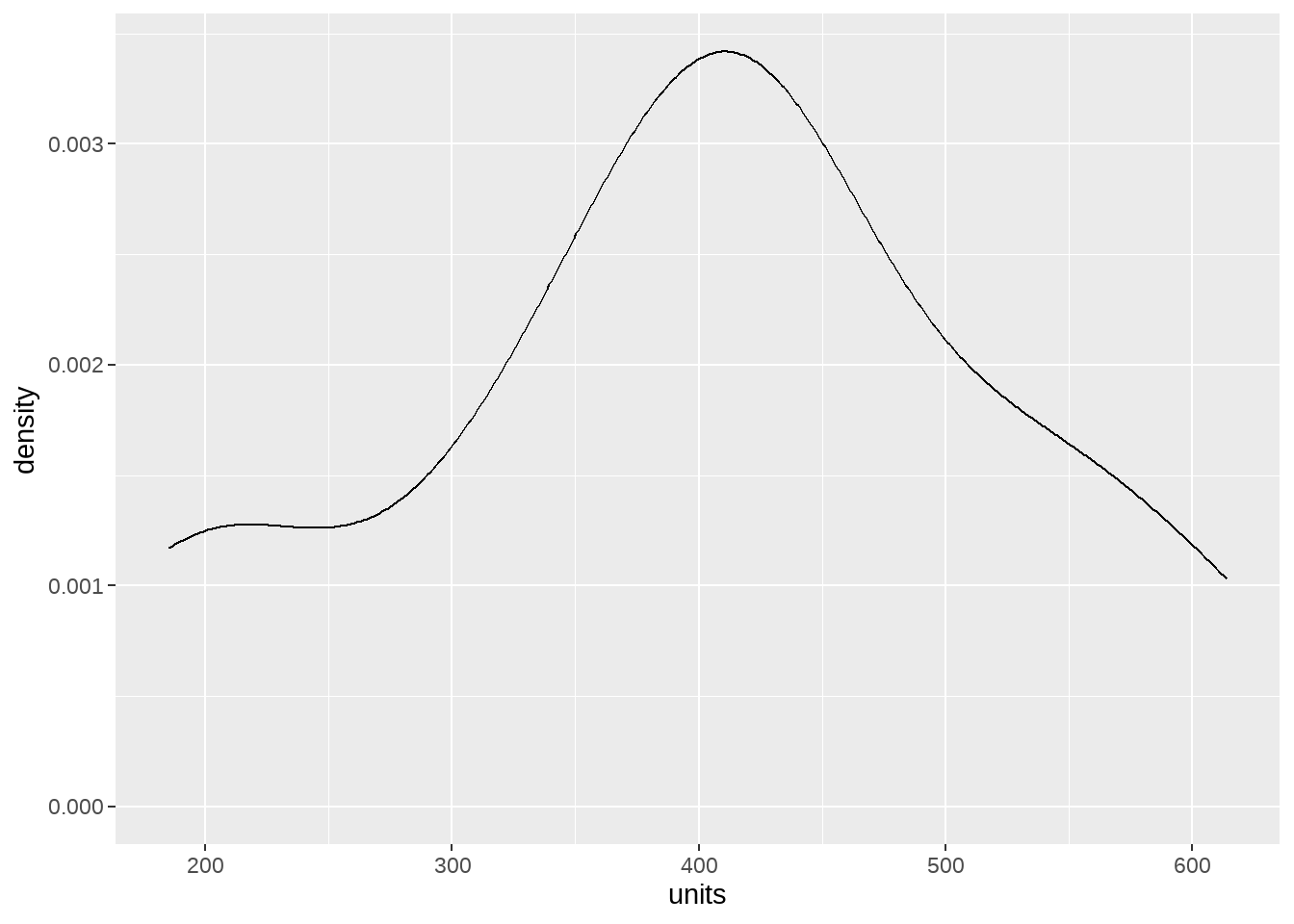
66.2.1 lm()
##
## Call:
## lm(formula = units ~ 1 + temp, data = icecream)
##
## Residuals:
##     Min      1Q  Median      3Q     Max
## -75.512 -12.566   4.133  22.236  49.963
##
## Coefficients:
##             Estimate Std. Error t value Pr(>|t|)
## (Intercept) -159.474     54.641  -2.919   0.0153 *
## temp          30.088      2.866  10.499 1.02e-06 ***
## ---
## Signif. codes:  0 '***' 0.001 '**' 0.01 '*' 0.05 '.' 0.1 ' ' 1
##
## Residual standard error: 38.13 on 10 degrees of freedom
## Multiple R-squared:  0.9168, Adjusted R-squared:  0.9085
## F-statistic: 110.2 on 1 and 10 DF,  p-value: 1.016e-06
confint(fit_lm, level = 0.95)## 2.5 % 97.5 %
## (Intercept) -281.22128 -37.72702
## temp 23.70223 36.47350
# Confidence Intervals
# coefficient +- qt(1-alpha/2, degrees_of_freedom) * standard errors

coef <- summary(fit_lm)$coefficients[2, 1]
err  <- summary(fit_lm)$coefficients[2, 2]

coef + c(-1,1)*err*qt(0.975,  nrow(icecream) - 2)
## [1] 23.70223 36.4735066.2.2 线性模型
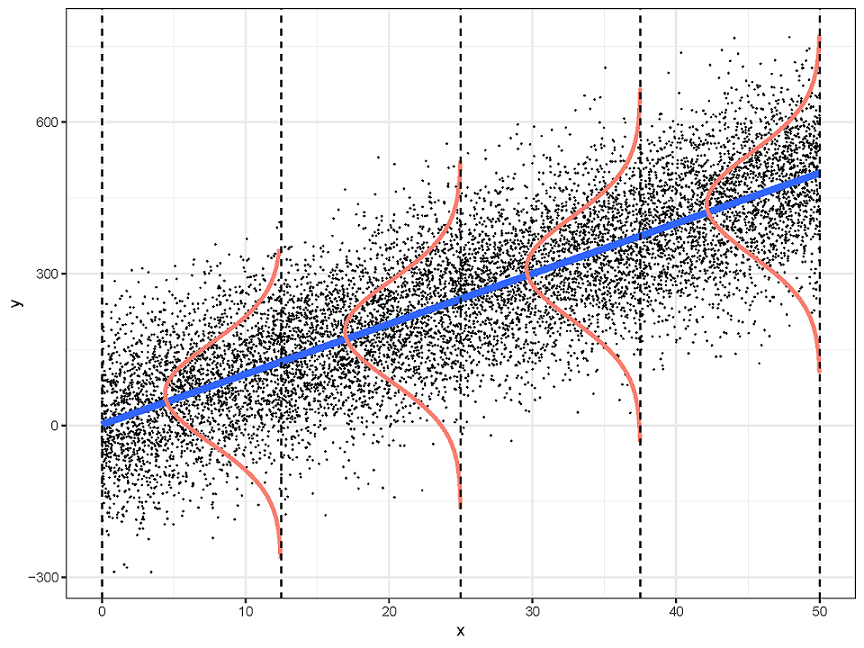
线性回归需要满足四个前提假设:
-
Linearity
- 因变量和每个自变量都是线性关系
-
Indpendence
- 对于所有的观测值,它们的误差项相互之间是独立的
-
Normality
- 误差项服从正态分布
-
Equal-variance
- 所有的误差项具有同样方差
这四个假设的首字母,合起来就是LINE,这样很好记
把这四个前提画在一张图中
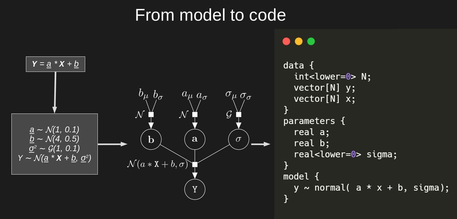
66.2.3 数学表达式
\[ y_n = \alpha + \beta x_n + \epsilon_n \quad \text{where}\quad \epsilon_n \sim \operatorname{normal}(0,\sigma). \]
等价于
\[ y_n - (\alpha + \beta X_n) \sim \operatorname{normal}(0,\sigma), \]
进一步等价
\[ y_n \sim \operatorname{normal}(\alpha + \beta X_n, \, \sigma). \]
因此,我们推荐这样写线性模型的数学表达式 \[ \begin{align} y_n &\sim \operatorname{normal}(\mu_n, \,\, \sigma)\\ \mu_n &= \alpha + \beta x_n \end{align} \]
66.3 stan 代码
stan_program <- "
data {
  int<lower=0> N;
  vector[N] y;
  vector[N] x;
}
parameters {
  real alpha;
  real beta;
  real<lower=0> sigma;
}
model {
  y ~ normal(alpha + beta * x, sigma);

  alpha  ~ normal(0, 10);
  beta   ~ normal(0, 10);
  sigma  ~ exponential(1);
}

"
stan_data <- list(
   N = nrow(icecream),
   x = icecream$temp,
   y = icecream$units
  )

fit_normal <- stan(model_code = stan_program, data = stan_data)- 检查 Traceplot
traceplot(fit_normal)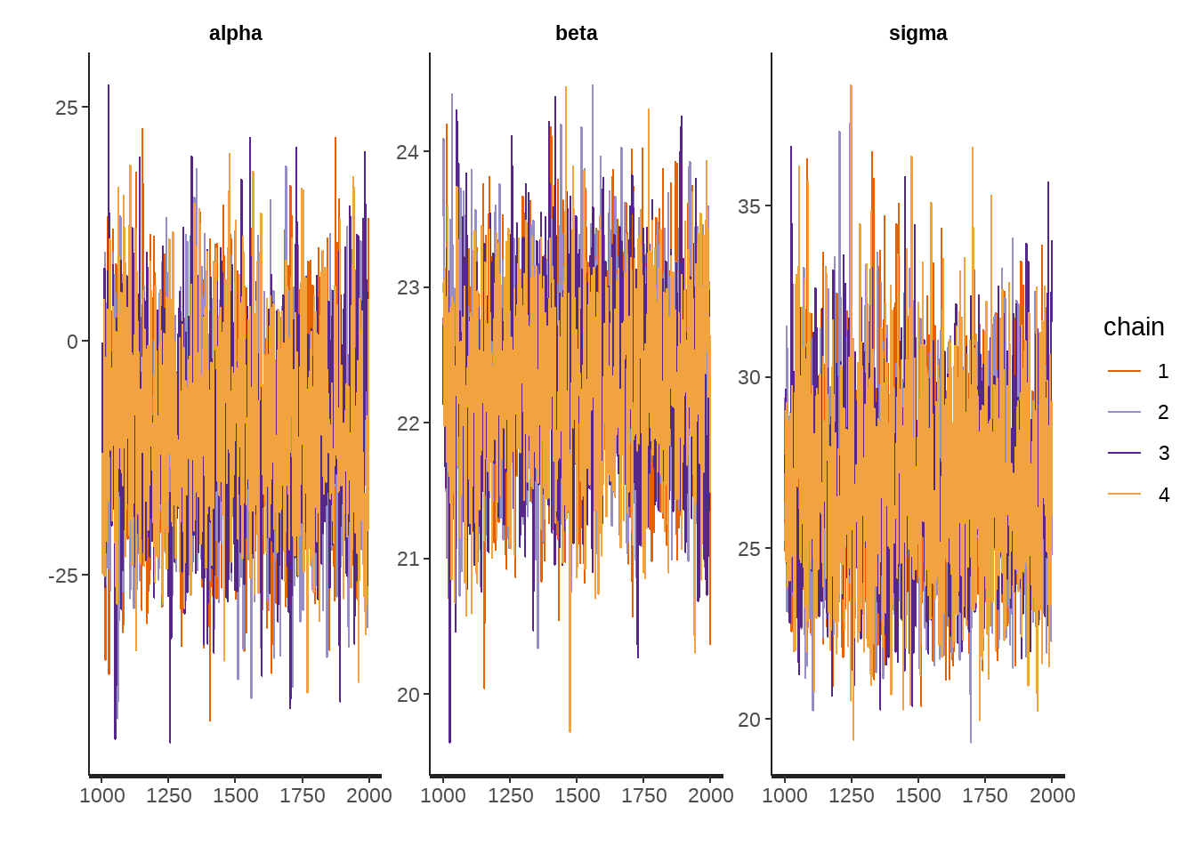
- 检查结果
fit_normal## Inference for Stan model: anon_model.
## 4 chains, each with iter=2000; warmup=1000; thin=1;
## post-warmup draws per chain=1000, total post-warmup draws=4000.
##
## mean se_mean sd 2.5% 25% 50% 75% 97.5% n_eff Rhat
## alpha -9.07 0.25 9.96 -27.75 -15.75 -9.32 -2.21 10.79 1609 1
## beta 22.33 0.02 0.66 21.06 21.88 22.32 22.79 23.58 1467 1
## sigma 26.86 0.06 2.70 22.06 24.92 26.69 28.58 32.53 2029 1
## lp__ -85.16 0.03 1.25 -88.50 -85.71 -84.85 -84.25 -83.75 1387 1
##
## Samples were drawn using NUTS(diag_e) at Mon Oct 28 09:47:47 2024.
## For each parameter, n_eff is a crude measure of effective sample size,
## and Rhat is the potential scale reduction factor on split chains (at
## convergence, Rhat=1).66.4 理解后验概率
提取后验概率的方法很多
-
rstan::extract()函数提取样本
post_samples <- rstan::extract(fit_normal)post_samples是一个列表,每个元素对应一个系数,每个元素都有4000个样本,我们可以用ggplot画出每个系数的后验分布
tibble(x = post_samples[["beta"]] ) %>%
  ggplot(aes(x)) +
  geom_density()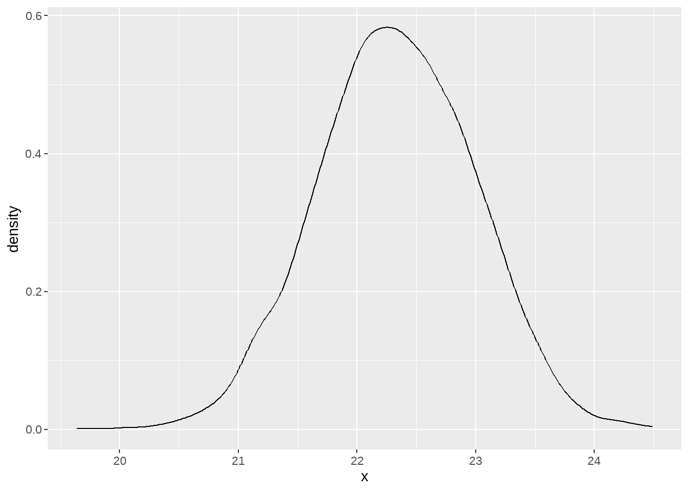
- 用
bayesplot宏包可视化
posterior <- as.matrix(fit_normal)

bayesplot::mcmc_areas(posterior,
                      pars = c("alpha", "beta", "sigma"),
prob = 0.89) 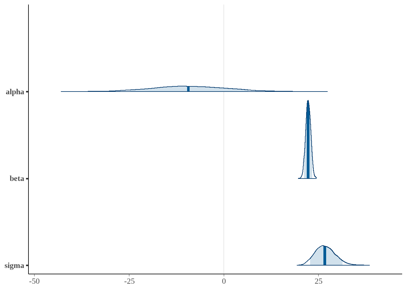
- 用
tidybayes宏包提取样本并可视化,我喜欢用这个,因为它符合tidyverse的习惯
fit_normal %>%
  tidybayes::spread_draws(alpha, beta, sigma) %>%

  ggplot(aes(x = beta)) +
  tidybayes::stat_halfeye(.width = c(0.66, 0.95)) +
theme_bw() 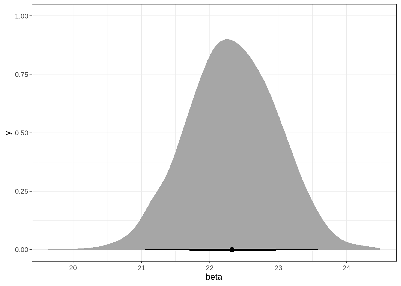
fit_normal %>%
  tidybayes::spread_draws(alpha, beta, sigma) %>%

  ggplot(aes(beta, color = "posterior")) +
  geom_density(size = 1) +

  stat_function(fun = dnorm,
        args = list(mean = 0,
                    sd = 10),
        aes(colour = 'prior'), size = 1) +
  xlim(-30, 30) +
  scale_color_manual(name = "",
                     values = c("prior" = "red", "posterior" = "black")
                     ) +
  ggtitle("系数beta的先验和后验概率分布") +
  xlab("beta")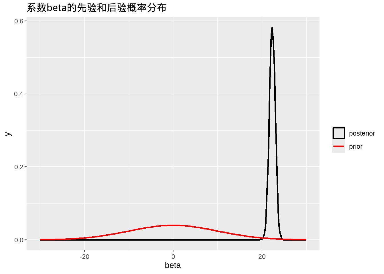
66.6 作业与思考
去掉stan代码中的先验信息,然后重新运行,然后与
lm()结果对比。调整stan代码中的先验信息,然后重新运行,检查后验概率有何变化。
- 修改stan代码,尝试推断上一章的身高分布
stan_program <- "
data {
  int N;
  vector[N] y;
}
parameters {
  real mu;
  real<lower=0> sigma;
}

model {
  mu ~ normal(168, 20);
  sigma ~ uniform(0, 50);

  y ~ normal(mu, sigma);
}

"

stan_data <- list(
  N = nrow(d),
  y = d$height
)

fit <- stan(model_code = stan_program, data = stan_data,
            iter = 31000,
            warmup = 30000,
            chains = 4,
            cores = 4
            )