9.7 Problem Set
- Table A provides metabolic rate, water loss, and fur and fat thicknesses for several species of animals. Using this information and Equations (9.10) and (9.11), calculate the maximum and minimum temperature differentials across the fat (\(T_b - T_s\)) and fur layers (\(T_s - T_r\)).
Rank the homeotherms from the highest to lowest difference between body temperature and surface temperature. Under what environmental conditions would an animal like to make this difference large? When would the animal like to make this difference small? What other mammals do you know of besides the pig that have thick fat layers? Why might this be? How does fat compare with fur or feathers as an insulation material? What is the relative efficiency of each? Is it clear now that the assumption that \(T_b\) ~ \(T_r\) for the lizard is not critical?
Table A
| M | \(E_{ex}\) | \(E_{sw}\) | \(d_b\) | \(d_f\) | ||||||
|---|---|---|---|---|---|---|---|---|---|---|
| Max. | Min. | Max. | Min. | Max. | Min. | Max. | Min. | Max. | Min. | |
| Shrew | 396 | 139 | 26 | 0 | 26 | 0 | 1 | 1 | 3 | 2 |
| Cow, summer | 104 | 104 | 9 | 4 | 58 | 6 | 14 | 14 | 5 | 5 |
| Cow, winter | 104 | 104 | 9 | 4 | 58 | 6 | 14 | 14 | 27 | 27 |
| Pig | 124 | 58 | 75 | 1 | 7 | 1 | 35 | 1 | 3 | 1 |
| Zebra finch | 213 | 91 | 91 | 22 | 0 | 0 | 1 | 1 | 3.5 | 3 |
| Locust | 600 | .07 | 14 | 0 | 0 | 0 | 1 | – | – | – |
| Cardinal | 107 | 77 | 77 | 3 | 0 | 0 | 2 | 1 | 15 | 5 |
| Jack rabbit | 77 | 63 | 63 | 9 | 0 | 0 | 2 | 1 | 15 | 8 |
| Fence lizard | 70 | – | 2 | – | – | – | 1 | – | – | – |
\(M\), \(E_{ex}\), \(E_{sw}\) in W m-2, \(d_b\) and \(d_f\) in m \(\times\) 10-3
- Construct the climate space of the pig, jack rabbit, and locust using the data presented below:
Table B
| \(M\) | \(E_{sw}\) | \(E_{ex}\) | \(d_f\) | \(d_b\) | \(T_b\) | ||
|---|---|---|---|---|---|---|---|
| Pig \(a_s=0.8\), \(M_b=120kg\) | I | 124 | 1 | 1 | 3 | 35 | 36 |
| II | 100 | 1 | 21 | 3 | 35 | 36 | |
| III | 69 | 7 | 66 | 1 | 10 | 37.5 | |
| IV | 58 | 7 | 75 | 1 | 1 | 41.7 | |
| Jack rabbit \(a_s=0.8\), \(M_b=2kg\) | I | 77 | 0 | 9 | 15 | 2 | 37.5 |
| II | 63 | 0 | 9 | 8.5 | 2 | 37.5 | |
| III | 43 | 0 | 12 | 8.5 | 2 | 38.5 | |
| IV | 45 | 0 | 20 | 7 | 1 | 39.5 | |
| V | 63 | 0 | 63 | 8 | 1 | 43.7 | |
| Locust \(a_s=0.8\), \(M_b=0.001kg\) | I | 600 | – | 14 | – | 1 | 42 |
| II | 600 | – | 14 | – | 0 | 20 | |
| III | 0 | – | 0 | 0 | 0 | 20 | |
| IV | 0 | – | 0 | – | 1 | 1 |
Spotila et al. (1973) were able to incorporate the effect of conduction. Thinking about the heat energy balance equation and assuming that the ground temperature is constant, how will the physiological limits be shifted?
Spotila et al. (1973) suggests that the area labeled A in the climate space of Figure 9.6 need not be included. Why might this be true? Are there any other areas like this? How does your answer compare with the information in Figure 9.3?
A comparison of the climate space diagrams in this module with those found in the Porter and Gates paper shows that the slopes of the lines are usually different under the same set of environmental and physiological conditions. This is because a different convection coefficient is used. Below is a table of weights and diameters for the same animals. Compute the convection coefficient in two ways: 1) using the formula that Porter and Gates (1969) provided; 2) using Mitchell’s (1976) relationship, assume \(V\) = 1.0 ms-1. Now make the comparison in a more systematic fashion; Let \(V\) = 0.1, 0.5, 1.0, 3.0, and 10 ms-1 and \(M_b\) = 0.00001, 0.001, 0.1, 1, 10 and 160 kg. Use the relationship between length and weight given in Appendix II to find a diameter corresponding to the weight values given. Compare the values by forming the ratio of Mitchell’s \(h_c\) divided by that of Porter and Gates.
| Animal | Diameter (m) | Body Mass (kg) |
|---|---|---|
| Sheep | 0.40 (fleece) | 70.0 |
| Cardinal | 0.050 | 0.020 |
| Lizard | 0.015 | 0.050 |
| Shrew | 0.018 | 0.010 |
- W. P. Porter (personal communication) has pointed out that Equations (9.10) and (9.11) apply to heat flow in a slab not a cylinder as shown in Figure 9.9. Derive the equation for heat flow through a cylinder (see Kreith 1973 or Ilatheway 1977) and through a plate of the same average area under steady state conditions. When will the two formulae give approximately the same result?
Compare this with the values used in Porter and Gates (1969) tabled below. Why does this work?
| Diameter D (cm) | Thickness of fur of feathers \(d_f\) (cm) | Thickness of fat layer \(d_b\) (cm) | |
|---|---|---|---|
| Desert iguana | 1.5 | 0.0 | 0.1 |
| Shrew | 1.8 | 0.3 | 0.1 |
| Zebra finch | 2.5 | 0.35 | 0.1 |
| Cardinal | 5.0 | 1.0 | 0.2 |
| Sheep | 25.0 | 12.8 | 0.1 |
| Sheep | 25.0 | 8.2 | 0.65 |
| Pig | 36.0 | 0.3 | 3.5 |
| Jack rabbit | 10.0 | 1.5 | 0.2 |
- Morhardt and Gates (1973) measured both the metabolic rate and the evaporative water loss as a function of effective ambient temperature These graphs are included below (Figures 9.13 and 9.14). We know that both these physiological parameters should also depend on the radiation levels and wind speeds. Consider the metabolic chambers to be equivalent to a blackbody environment and then plot-lines of constant metabolic rate and evaporative rates on the climate space diagram (let \(M_b\) = 0.2 kg, \(V\) = ms-1). Now repeat this process on the climate space of Figure 9.3. What are times of environmental stress? What might be the preferred activity period of the animal? Remember that the metabolic curve is for a resting and fasting animal. How does that change your answer? Consult the original paper and investigate what other thermal microhabitats were available. Is it critical that we do not have any information about the animal in its burrow?
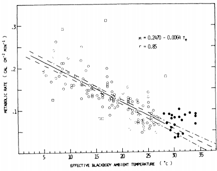
Figure 9.13: Metabolic rates of all squirrels used in this study as a function of effective ambient temperature. Open circles represent metabolic rates of resting squirrels at effective ambient temperatures below the thermal neutral zone. Closed circles represent metabolic rates of resting squirrels at effective ambient temperatures above the lower critical temperature of 28°C. Open squares represent meta bolic rates of exceptionally active squirrels, or those whose body temperature was falling below normal levels. The solid line is a least squres regression line fitted to the open circles, and the broken lines delineate the 95 percent confidence interval of the least squares line. The equation of the line and the correlation coefficient (r) are shown.
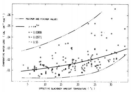
Figure 9.14: Evaporative water loss as a function of effective temperature (corrected to 4 mg 820/liter air). The data collected at different relative humidities have been corrected to a constant relative humidity (vapor density = 4 mg 820/liter air) A logistic curve is fitted to the data, and the correlation coefficient (r) is shown.