15.4 Solar Radiation
The microclimate model used to generate these layers includes a solar radiation sub-module that computes solar radiation reaching flat ground on the basis of time, longitude and latitude, and atmospheric properties including gridded cloud and aerosol (dust) data. The computation starts by determining the extra-terrestrial radiation reaching the outer atmosphere, given the location, day of the year and hour of the day. It then determines how that radiation is attenuated as it passes through the atmosphere to hit the ground.
Let’s take a look at some of the data. We will again use the ‘raster’ package of R, and you’ll also need to have installed the ‘ncdf4’ package, because the data is stored in netCDF format as was the case for the soil temperature data from Prac 1.
library(raster)
# put your path here for microclim data folder
path<- 'microclim_Aust/'

month<-1 # choose which month you want, 1 or 7 (i.e. Jan or Jun)
# read the file into memory
solar<-brick(paste0(path,"solar_radiation_Wm2/SOLR_",month,".nc"))
The paste command combined our microclimate data path, the name of the folder holding the data, and then the month we wanted, thus specifying the file “microclim_aust/solar_radiation_Wm2/SOLR_1.nc”. We use the brick function of the ‘raster’ package to load this multi-layer file. There are 24 layers, one for each hour of the day. Let’s plot the first one - in the plot command we can specify this using double square brackets.
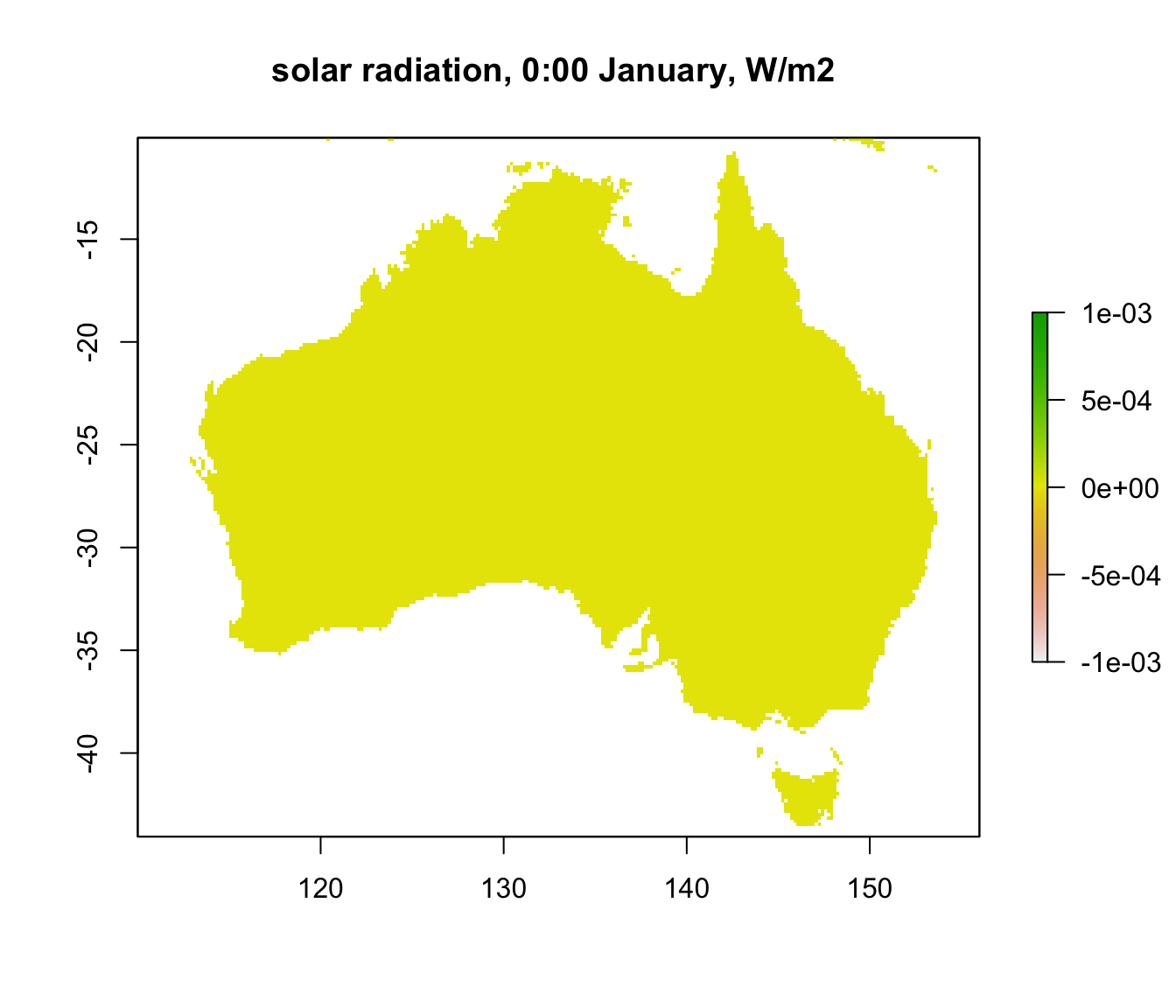
Well, that’s not very interesting is it? This is because we plotted layer 1 which is midnight. Let’s plot layer 13, which is 12 noon, instead.

Now we can see a wide range of values, from near 1000 \(W\:m^{-2}\) in central Australia down to just over 700 in the far north and south of the country. You can clearly see the effect of cloud cover during the wet season in the ‘Top End’ of Australia.
You may have also noticed the somewhat blocky appearance of the layer. This is because the aerosol and cloud cover layers are a coarser resolution than the rest of the input grids. In fact, there is a big increase in the aerosol grid (and hence decrease in the solar radiation) over central Australia which has been manually reduced in this data set from the original microclim data set.
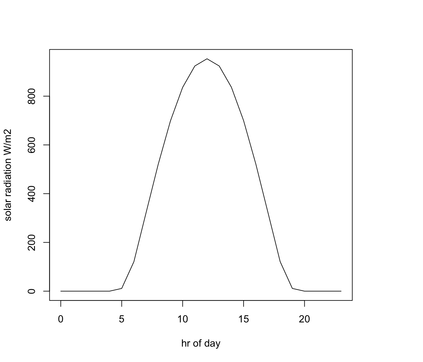
Now let’s extract and plot 24 hours of data from a particular location. We’ll use the same location we used in Prac 1, i.e. a place in the Flinders Ranges of South Australia. First we’ll plot the chosen location on the map. Then, we once again use the ‘raster’ package function extract, which we met in Prac 1, to get the data for that point across all 24 layers.
lon.lat = cbind(138,-32) # define the longitude and latitude
points(lon.lat, cex=1.5, pch=16, col='black') # note that cex specifies the point size 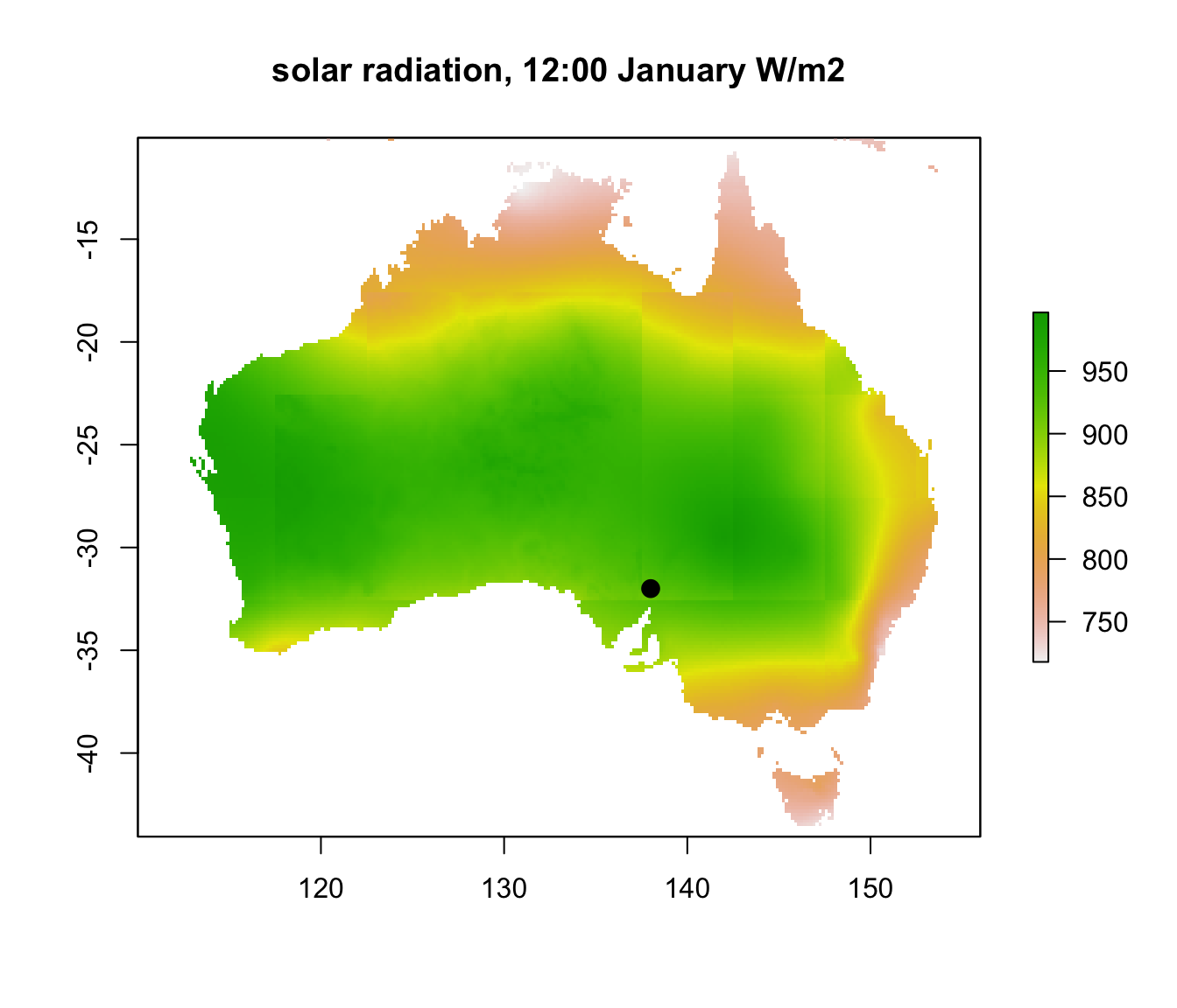
# extract data for all layers in 'solar' at location 'lon.lat'
solar.hr = extract(solar, lon.lat)
solar.hr = t(solar.hr) # transpose the values, in preparation for the plot command
hrs = seq(0,23) # create a sequence of hours
# plot solar radiation as a function of hour, as a line graph (using type = 'l')