16.6 Mapping the heat limit of the Desert Iguana
Now we will repeat the procedure and map the heat limits for the Desert Iguana, but this time in the hottest month, July. Note that we will use the minimum absorptivity observed for the Desert Iguana of 0.6 rather than 0.8 that we used for the cold limit.
# choose the high temperature (45 degrees C) parameters
a_min <- pars$abs_min[5] # get the minimum solar absorptivity value, choosing row 5
D <- pars$D[5] # diameter, m
T_b_upper <- pars$T_b[5] # body temperature, deg C
M <- pars$M[5] # metabolic rate, W/m2
E_ex <- pars$E_ex[5] # evaporative heat loss from respiration, W/m2
E_sw <- pars$E_sw[5] # evaporative heat loss from sweating, W/m2
k_b <- pars$k_b[5] # thermal conductivity of the skin, W/(m C)
K_b  <- k_b/pars$d_b[5] # thermal conductance of the skin, W/(m2 C)

# choose the July wind speed and air temperature
V <- wind_jul_NAm # wind speed, m/s
T_air<-Tair_jul_NAm # air temperature range to consider, degrees C

# compute the total radiation load for each air temperature and wind speed combination that would
# give a Tb of 45 degrees, the upper survivable limit
Q_abs_upper <- Qabs_ecto(D = D, T_b = T_b_upper, M = M, E_ex = E_ex, E_sw = E_sw, K_b = K_b, epsilon = epsilon, T_air = T_air, V = V)

# subtract available radiation from required for 45C degrees Tb
enbal_hot <- Q_rad_jul_NAm - Q_abs_upper
Now we can plot the results for the heat energy budget at the upper thermal limit. Now, where the ‘enbal_hot’ layer is positive, it means the radiation load on the lizard at that site in the open would exceed that which would result in a body temperature of 45 at the particular wind speed and air temperature at that location.
# plot the results
plot(enbal_hot[[5]], main = "energy balance (W/m2), 4am January", zlim = c(-1500,0))
map('world', add = TRUE)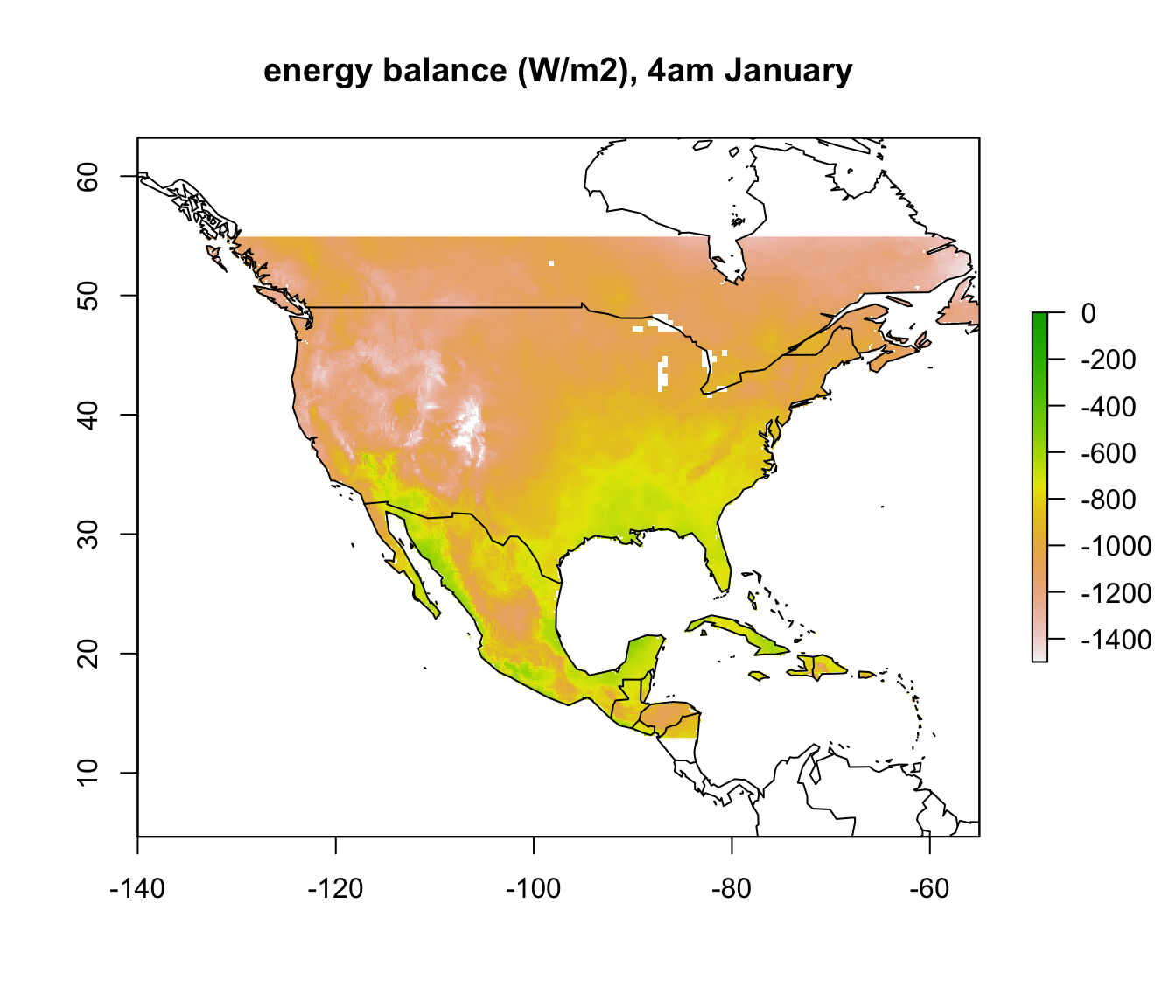
plot(enbal_hot[[13]], main = "energy balance (W/m2), 12pm January", zlim = c(-1500,0))
map('world', add = TRUE)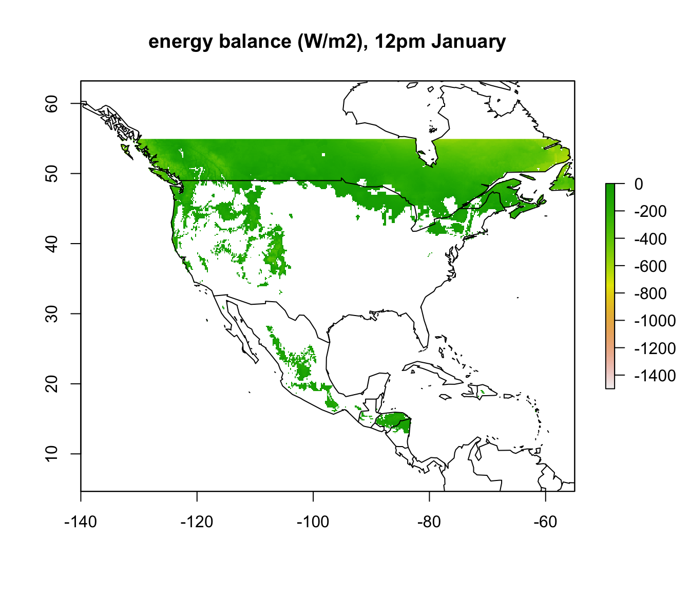
To summarise our calculations so far, let’s make our results binary with values of 1 for pixels that are inside the climate space limits and 0 for pixels that are outside. We’ll use the ifelse native R function together with the ‘raster’ function values which together allow you to conditionally replace values in a raster. We will then make a final result brick called ‘enbal’ where we multiply the two sets of rasters together so you can see at what times and places they would be both above their lower thermal limit and below their upper thermal limit, considering both January and July.
enbal_hot_binary <- enbal_hot
# replace values greater than zero, i.e. where there is too much radiation available to match
# the level  needed to produce a 45 degree C body temperature for each wind speed and air
# temperature combination across North America, otherwise give value 1
values(enbal_hot_binary) <- ifelse(values(enbal_hot) > 0, 0, 1)

enbal_cold_binary <- enbal_cold
# replace values greater than zero, i.e. where there isn't enough radiation available to match
# the level needed to produce a 3 degree C body temperature for each wind speed and air
# temperature combination across North America, otherwise give value 1
values(enbal_cold_binary) <- ifelse(values(enbal_cold) > 0, 0, 1)

enbal = enbal_hot_binary * enbal_cold_binary
If you install the ‘animate’ package in R, you can check out the results as an animation. You’ll have to click the stop button on the console window to stop the animation when you’re finished admiring your work.
library(animation)
times <- paste0(seq(0,23),":00 hrs") # sequence of labels of hours of the day
animate(enbal, main = times)
Now we’ll sum the final raster brick to get the total number of hours the Desert Iguana would spend inside its climate space in open habitat and then add the distribution points to this map.
sumembal=sum(enbal) # sum the total number of hours within climate space at at each site

# first plot without the distribution records, so you can see the results clearly
plot(sumembal, main = "Total hours spent within climate space")
map('world', add = TRUE)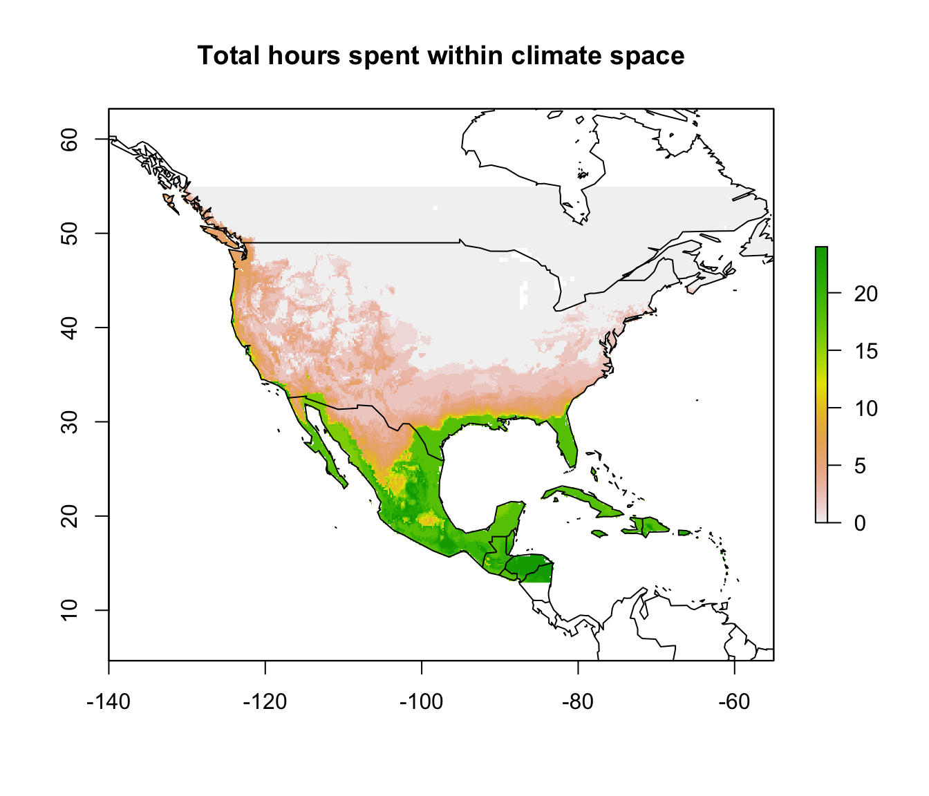
# now plot again with the distribution records
plot(sumembal, main = "Total hours spent within climate space")
points(dipso_dist$lon, dipso_dist$lat, col = "black", cex = 0.5)
map('world', add = TRUE)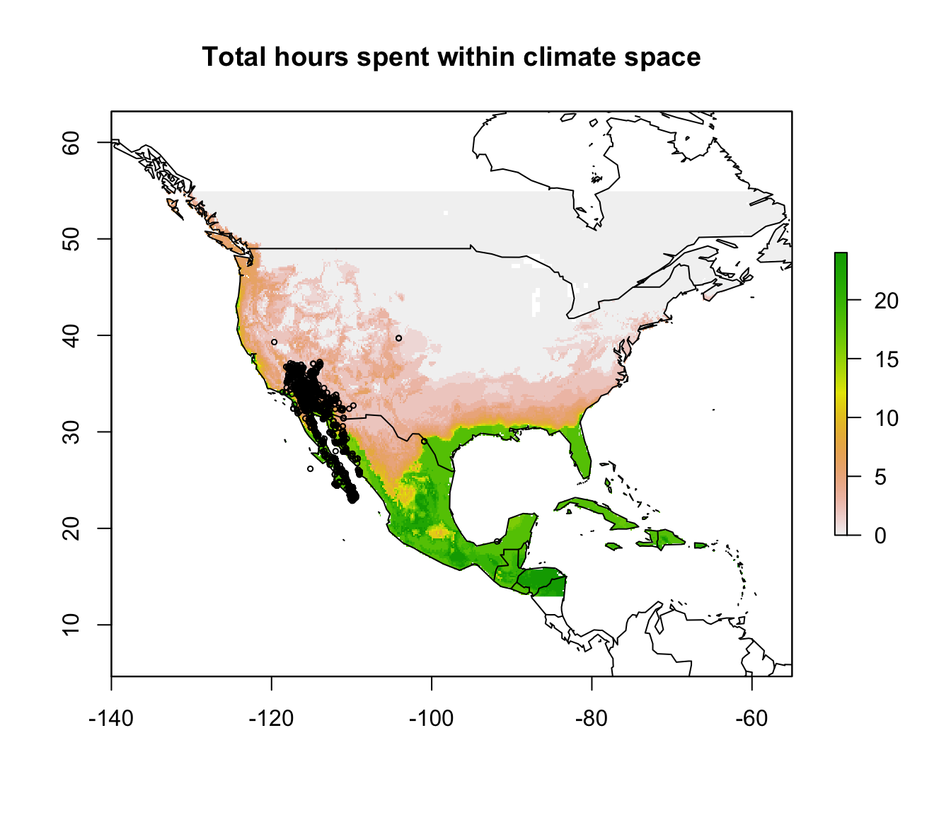
What can you say from this analysis about the distribution limits of this lizard? Have you identified any areas as definitely outside the fundamental or ‘thermodynamic’ niche of this species?