13.5 Use of the Heat Conduction Equation

Experience with actual temperature data indicates that with the assumption of a constant diffusivity, Equation (13.8) describes in a general way the phenomenon of soil heat flow and resultant temperature distribution. It is the goal of this section to investigate in more detail the utility of this formalized approach through an analytical solution of Equation (13.8).

13.5.1 Boundary Conditions

Hatheway (1977b) discusses in general the need for well-posed boundary conditions in order to derive a unique solution for a diffusion type equation (such as our Equation 8). It turns out that it is necessary to specify \(T(z,t)\) or \(\frac{\partial T}{\partial z}\)at the soil surface (z=0), and at some depth in the soil, which we take as \(z=\infty\). This latter choice is based on the observation that the soil temperature at substantial depths, say greater than 10 meters, is practically constant. Hence, our lower boundary condition is simply

\[\begin{equation} T(\infty,t)=\overline{T} \tag{13.9} \end{equation}\] where the overbar signifies the average temperature, which we will assume constant with depth. For the upper boundary condition, we will make the assumption that the diurnal (Fig. 13.2) or annual (Fig. 13.9) variation of surface temperature can be approximated by a sine wave. This is a somewhat better approximation for annual than diurnal variations. We choose the time scale such that when \(t=0\) the surface temperature is \(\overline{T}\). The upper boundary condition then becomes

\[\begin{equation} T(0,t)=\overline{T}+A(0)\sin\omega t \tag{13.10} \end{equation}\]

For the diurnal case, the period of oscillation is 24 hours, or 86,400 seconds. Of course, the \(\omega\) is angular frequency and can be written \[\omega = 2\pi/86,400=7.27(10)^{-5}second^{-1}\] The argument of the sine function \((\omega t)\) is then expressed in radians if \(t\) is in seconds. \(A(0)\) is the amplitude of the temperature wave at the surface, so that \(T(0,t)\) over the course of a day varies between \(\overline{T}-A(0)\) and \(\overline{T}+A(0)\).

Problem Solution The solution of Equation (13.8) which satisfies boundary conditions (13.9) and (13.10) is

\[\begin{equation} T(z,t)=\overline{T}+A(z)\sin[\omega t+B(z)] \tag{13.11} \end{equation}\] The reader is referred to Carslaw and Jaeger (1959) for the mathematical details. Now \(A(z)\) and \(B(z)\) represent the amplitude and phase lag of the temperature wave, respectively. From our earlier discussion of Fig. 13.2, we expect \(A(z)\) and \(B(z)\) to be decreasing and increasing functions of depth, respectively. By substituting our solution (13.11) into the differential Equation 13.8, we find that

\[\begin{equation} A(z)=A(0)exp(-z/D) \tag{13.12} \end{equation}\] and

\[\begin{equation} B(z)=-z/D \tag{13.13} \end{equation}\]

where \(D\) is termed the damping depth, and is related to the thermal properties of the soil and the frequency of the temperature wave by the expression

\[\begin{equation} D=(2K/\omega)^{1/2} \tag{13.14} \end{equation}\]

Several aspects of this solution (Equations (13.11) through (13.14)) will now be discussed in detail.

13.5.2 Properties of the Harmonic Solution

Since the temperature is a function of both \(z\) and \(t\), it is useful in looking at graphical representations to present two sets of curves. As is immediately apparent from Equation (13.11), a plot of \(T\) versus \(t\) for various depths produces a family of sinusoids:

# Variation of temperature across time with depth

w= 2*pi/86400 #s^-1, angular frequency
k= 0.0042 #thermal conductivity of soil, cal cm^-1 s^-1 °C^-1
C= 0.5 #volumetric heat capacity, cal cm^-3 °C^-1

#Estimate aggregate parameters
K= k/C #thermal diffusivity
D= (2*K/w)^0.5 #damping depth, cm
  
Tbar= 20 #°C
A0= 8 #°C

#z in depth in cm
#sec in time in seconds
Tsoil= function(z,sec) {
A= A0*exp(-z/D)
B= -z/D
Tbar + A*sin(w*sec+B)
}

sec=(0:23)*60*60 #hr

#plot across depths
plot(sec/(60*60),Tsoil(0,sec), type="l", lty="dashed", 
     xlim=c(0,24), xlab= "Time (hr)", ylab="Temperature (°C)")
points(sec/(60*60),Tsoil(5,sec), type="l", col="skyblue")
points(sec/(60*60),Tsoil(10,sec), type="l", col="skyblue2")
points(sec/(60*60),Tsoil(20,sec), type="l", col="skyblue3")
points(sec/(60*60),Tsoil(40,sec), type="l", col="skyblue4")
abline(h=20)
legend("topright", c("z=0cm","z=5cm","z=10cm","z=20cm","z=40cm"), 
       col=c('black','skyblue','skyblue2','skyblue3','skyblue4'), 
       lty=c('dashed', rep('solid',4)), bty = "n")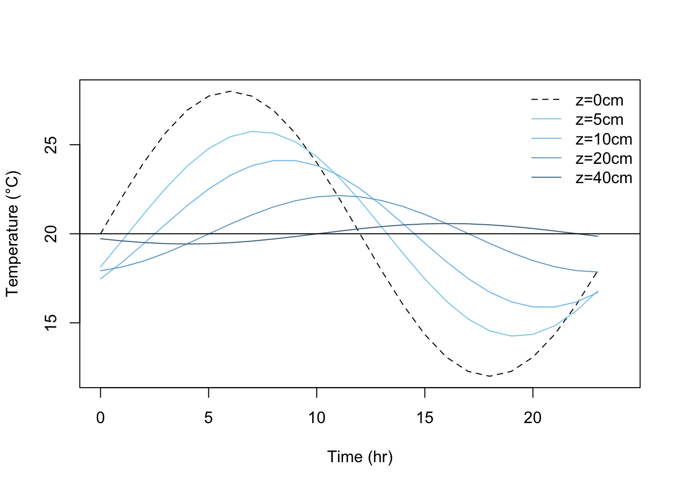

Figure 13.10: Variation of temperature with depth for a sand soil. A value of \(k=0.042calcm^{-1}sec^{-1}C^{-1}\) and \(C=0.5cal cm^{-3}C^{-1}\) has been assumed resulting in a damping depth D=15.2cm

Notice the similarities between this and some actual measurements (Figs. 13.2 and 13.9). In general, these figures exhibit similar amplitude reductions and phase lags with depth (see section 2) whose characteristics are attributable to the functions \(A(z)\) and \(B(z)\) in our solution. The amplitude exhibits exponential decay (Equation (13.12)), a phenomenon common to many situations in chemistry, biology and economics, to name just a few. Notice that \(A(D) = e^{-1}A(0) = 0.37A(0)\), so that the amplitude of the temperature wave at \(z = D\) is 37 percent of its surface value. Similarly, at \(z = 4.46 D\), we find a 99 percent amplitude reduction. The phase lag is embodied in the function \(B(z)\), which is a simple linear function of \(z\). For example, when \(z = \pi D\), \(B(z) = -\pi\), so the maximum (or minimum) at depth \(z = \pi D\) is exactly out of phase with the corresponding extreme of the temperature wave at the surface. For example, in the plot above, \(\pi D=\pi\cdot15.2=47.8cm\), and we find the 40 cm wave to be almost out of phase with the surface wave, as expected.

A plot of \(T\) versus \(z\) for various times of day using the same values of \(\overline{T}\), \(A(0)\), and \(D\) as for the figure above produces the following family of curves. As was mentioned in section 3 while discussing Fig. 13.8, we can deduce the direction of heat flow for this type of plot by the curvature of the temperature profile. Here again the damping of the temperature wave with depth is apparent.

# Soil temperature profiles
w= 2*pi/86400 #s^{-1}, angular frequency
D= 12.2 #damping depth, cm
Tbar= 20 #°C
A0= 8 #°C

Tsoil= function(z,sec) {
A= A0*exp(-z/D)
B= -z/D
Tbar + A*sin(w*sec+B)
}

#z in depth in cm
#sec in time in seconds
z= 0:40 #depths, cm

sec=(0:23)*60*60 #hr

#plot across depths
plot(Tsoil(z,2*60*60),z, type="l", col="skyblue", xlim=c(10,30), 
     ylim=c(40,0), xlab= "Temperature (°C)", 
     ylab="Soil depth measured from surface (cm)")
points(Tsoil(z,6*60*60),z, type="l", col="skyblue1")
points(Tsoil(z,10*60*60),z, type="l", col="skyblue2")
points(Tsoil(z,14*60*60),z, type="l", col="skyblue3")
points(Tsoil(z,18*60*60),z, type="l", col="skyblue4")
points(Tsoil(z,22*60*60),z, type="l", col="darkblue")
legend("bottomright", c("hr=0200","hr=0600","hr=1000","hr=1400", 
                        "hr=1800","hr=2200"), 
       col = c('skyblue', 'skyblue1','skyblue2','skyblue3',
               'skyblue4', 'darkblue'), lty="solid", bty = "n")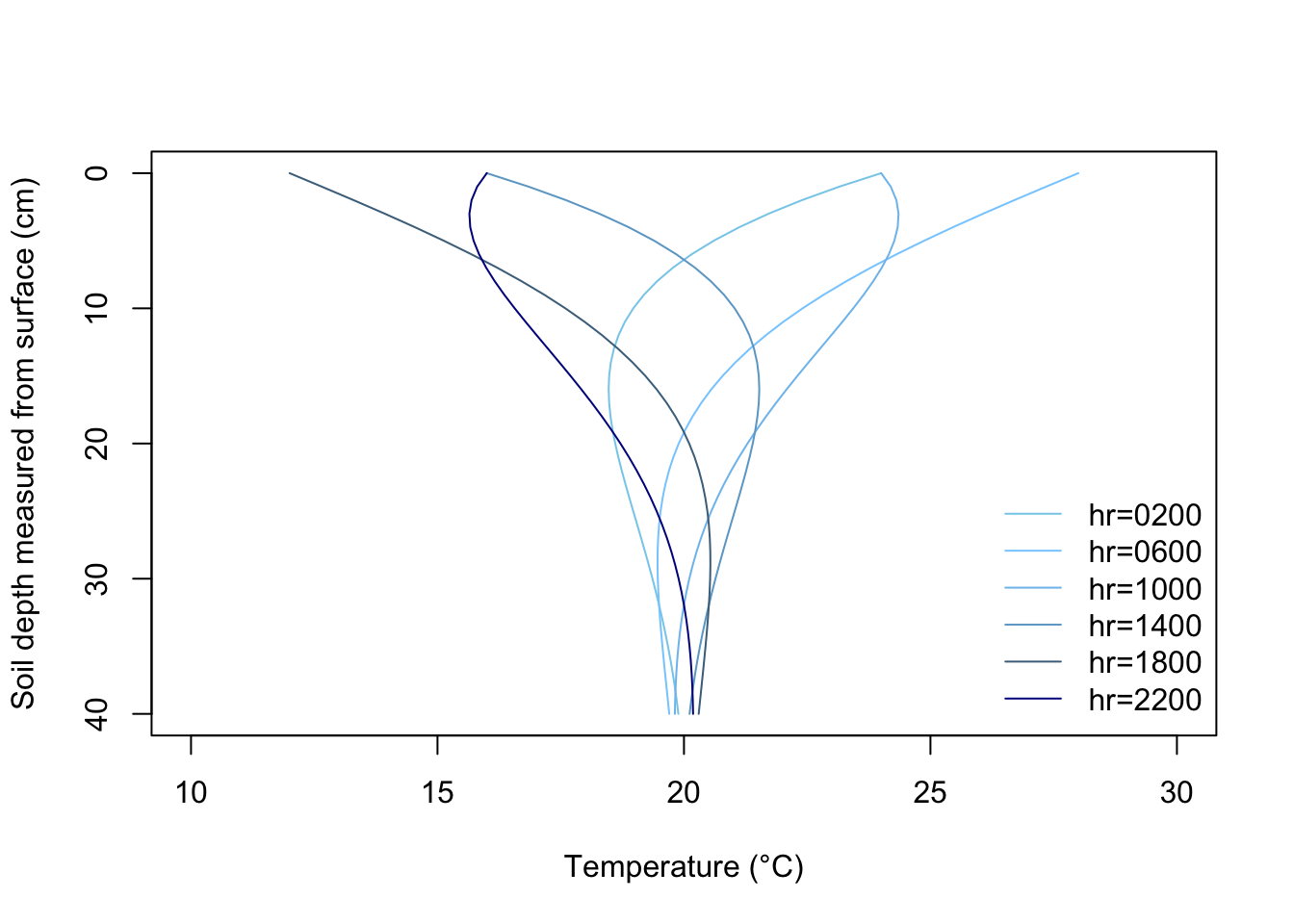

Figure 13.11: Plot of soil temperature versus depth for various times of day, derived from Equations 11 through 13. Assumed values for the various constants were D=12.2cm, \(\bar T\)=20°C, and A(0)=8°C.

13.5.3 Comparison of Theory with Experiment

In the process of formulating a closed form solution for soil heat flow which described at least the general state of affairs in the soil profile, we made several assumptions. The acid test, of course, of the quality of these assumptions is how well our simplified solution (i.e., Equations (13.11)-(13.14)) reflects reality. Comparison of the time series we plotted in R (figure 13.10) with figures 13.2 or 13.9 and the soil temperature profile (figure 13.11) with figure 13.12 indicate that general agreement is found. Minor discrepancies do occur, and it is instructive to examine these in light of our prior assumptions (section 3).

First of all, however, an examination of our upper boundary condition reveals an obvious difficulty in that it applies well only under clear sky conditions. Variable weather conditions as well as vegetation cover can lead to substantial deviations from a sinusoidal surface temperature variation (Fig. 13.13). The more general case of a periodic surface temperature variation that is not a simple time function can be handled by a technique called Fourier analysis. In addition, it is possible to deal with small systematic nonperiodic variations superimposed upon a larger periodic variation. Treatment of these refinements is available in Van Wijk and DeVries (1966).

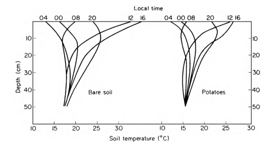
Figure 13.12: Diurnal change of soil temperature measured below a bare soil surface and below potatoes (from Monteith 1973).

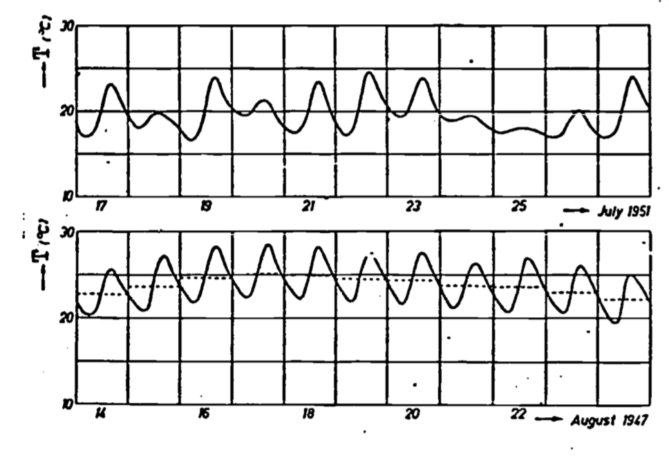
Figure 13.13: Soil temperature variations at 10 cm depth in a clay soil under a short grass cover at Wageningen, the Netherlands. The upper curve shows large deviations from a periodic function owing to variable weather conditions, while the lower curve corresponding to a sequence of bright days has a periodic character. The average daily temperatures are indicated by the dotted lines which have been drawn such that they divide the surfaces bounded by the temperature curves for each day equally (from Van Wyjk 1966).

Variation of thermal properties (characterized by diffusivity) with position, temperature and time are generally secondary to the above effects concerning the upper boundary condition. Temperature effects are slight and usually ignored. Variation with depth can be dealt with by use of a multilevel model (Van Wijk and Derksen 1966), while time variation can be treated by considering diffusivity as a function of time when solving Equation (13.8) (Van Wijk and DeVries 1966). Both these latter effects are caused in most part by the changes in moisture content of the soil, which is generally a function of both depth and time (Fig. 13.14). DeVries (1975) discusses the problem of combined heat and moisture transfer. We have discussed these effects in relation to conductivity (Fig. 13.6) and diffusivity. Of course, variation of diffusivity with depth occurs also as a result of layered soils and/or differences in soil density (and thus volumetric heat capacity) caused by compaction or tillage.

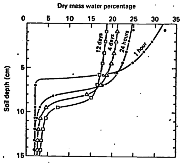
Figure 13.14: Soil water profiles at various times after water was added at the soil surface (from Taylor and Ashcroft 1972).

Analogous, but somewhat more complex due to accounting for transient dynamics, soil temperatures models are available in TrenchR.

13.5.4 Application of Results

A major use of the quantitative solution discussed here, and of the possible refinements mentioned, is to explain and illustrate how the temperature distribution of, the soil is determined. For a bare soil under clear skies, our solution approximates reality quite well. Variable weather, vegetative cover, various soil inhomogeneities (including changing moisture content) as well as moisture movement (liquid and vapor) can further complicate attempts at solution. As indicated in the previous paragraph, some types of inhomogeneity can be handled by extension of the present analysis. The upper boundary condition can be modeled using Fourier analysis. Alternatively, since the temperature of the soil surface ultimately is a result of the partitioning of solar energy into evaporation, heating of the air and heating of the soil, we may first calculate \(G(0)\), and from this obtain \(T(0)\). However, this requires modeling of the energy balance (see e.g., Hatheway 1977a, Stevenson 1977a, b, c). In practice, it may be easier to measure soil temperature and heat flux directly rather than deal with the further complexities of the energy balance and surface layer of the atmosphere.

In some cases, however, conditions may be close enough to ideal so that the simple model described here can give quite useful results. For example, Mitchell et al. (1975) present the results of a microclimatic model for dry desert-like areas with sparse vegetation. A finite difference scheme is used to solve the soil heat co-conduction equation. In an attempt to simplify the model, constant diffusivity and soil water content was assumed, and changes of state (i.e., evaporation) were ignored. Standard Weather Bureau data input were solar radiation and average monthly air temperature. The former parameter sets the upper boundary condition while the latter approximates the soil temperature at 0.6 m. (From our discussion of damping depth, it should be clear that there is little diurnal temperature change in the soil at 0.6 m depth.) Comparison of model prediction with actual measurements indicate that soil temperatures determined by both methods agreed within \(\pm2\)°C for daily variations of from 15°C to 35°C. Apparently, then, even simplified models of soil thermal behavior as discussed in this module would seem to have practical application in environmental modeling. Certainly simple models must serve as the basis of more comprehensive schemes leading to more complete understanding of the affected biological processes.