13.4 Formal Development
In the preceding section, a cause and effect relationship between soil heat flow and temperature distribution was implied. It is instructive to formalize this relation; indeed, the equation doing so will form the basis for subsequent discussion. First of all, however, it is necessary to present a more rigorous specification of the problem.
13.4.1 Fourier’s Law of Heat Conduction
Van Wijk and DeVries (1966) present a good discussion of the simplifying assumptions made to facilitate the mathematical development of heat conduction. These include:
The soil is homogeneous with respect to heat transfer by conduction. Now, conduction of heat is due to the transfer of the random vibratory motion of the molecules in the medium. Due to the natural variety of the soils, one would consequently not expect homogeneous soil heat transfer. However, if the soil thermal properties considered are bulk values, i.e., averaged over a volume of soil that is large with respect to the inhomogeneities, then this is a good assumption. It has the effect of making the heat transfer at any point independent of position.
Heat flow takes place only in the vertical direction. Since the heat input due to solar radiation can be considered uniform at the surface, this assumption is not limiting for a horizontally homogeneous surface.
There are no sources or sinks for heat (such as by chemical reaction) nor conversion of heat, into other forms of energy (such as latent heat of evaporation).
Hence the problem we are considering can be termed unidirectional heat conduction in a homogeneous medium. Empirical observation of this phenomenon leads to the conclusion that the heat flow between two points in such a medium is proportional to the temperature difference between those points. Such an observation seems consistent with our personal experience; the hotter the burner on the stove, the faster the kettle heats up. Of course, if a kettle of water is allowed to reach the boiling point, then further heat input is utilized to vaporize the water without further temperature increase. This is why we have included assumption 3.
Consider a block of soil (Fig. 13.4. The amount of heat energy which flows by conduction (\(Q\)) is directly proportional to the temperature difference (\(\Delta T\)) between top and bottom faces, as we have said before. We can write:
\[\begin{equation} Q\varpropto\Delta T \tag{13.1} \end{equation}\] The amount of heat transmitted through the soil block per unit time (\(t\)) is termed the heat flux (\(Q/t\)). The heat flux per unit area (\(A\)) is termed the heat flux density (\(Q/At\)). The heat, or heat flux density (also termed \(G\)), has also been observed to be proportional to \(\Delta T\), while being inversely proportional to the length of the path (\(L\)).
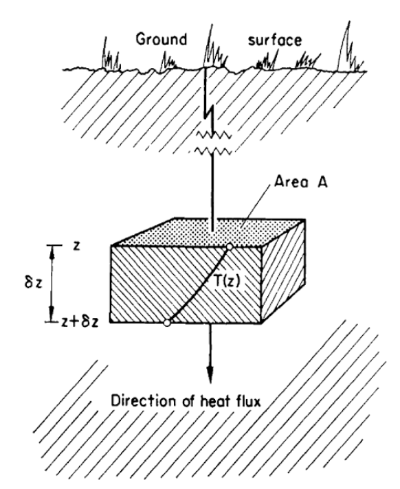
Figure 13.4: One dimensional heat conduction (from Rose 1966).
Therefore one can write
\[\begin{equation} G=\frac{Q}{At}=-k\frac{\Delta T}{L} \tag{13.2} \end{equation}\] where the constant of proportionality (\(k\)) is the thermal conductivity. In fact, Equation (13.2) can be considered a defining relation for thermal conductivity. If we now adopt the standard procedure of calculus and consider small changes in temperature (\(dT\)) over small increments of time (\(dt\)), one gets the standard form of Fourier’s law of heat conduction:
\[\begin{equation} G=-k\frac{dT}{dz} \tag{13.3} \end{equation}\]
It is important to notice the introduction of the minus sign. In words, this simply means that the direction of heat flow is opposite to the direction in which the temperature increases. To illustrate this, consider Fig. 13.5, where we assume that soil temperature varies linearly with depth in the soil. Observe the opposite sense of temperature change and heat flux density. Alternatively, one may deduce the sign from consideration of the temperature gradient \((\frac{dT}{dz})\), or slope, of the \(T\) versus depth (\(z\)) curve. As the depth increases, the temperature decreases. Hence the temperature gradient \(dT/dz\) is negative. For downward heat flux to be positive, which is the usual convention, we must add the minus sign to obtain Equation (13.3) (see also symbols, units, and dimensions in Table A in Appendix).
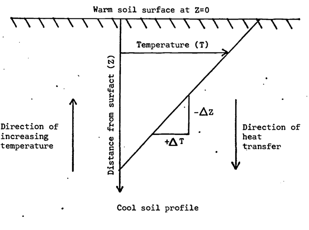
Figure 13.5: Illustration of the source of the minus sign found in Fourier’s law of heat conduction (Equation 13.3)
Equation (13.3) clearly indicates the importance of the thermal conductivity in determining the magnitude of the heat flux density. Consequently, we wish to understand what factors affect its value. If \(dT/dz = 1\) in Equation (13.3), then the thermal conductivity has the interpretation of the flux density in response to a unit gradient. In such terms one can compare typical values of thermal conductivity for various materials, gaining a feel for their relative ability to conduct heat (Table 13.1). Such comparison reveals that the average thermal conductivity of soil is not only a function of mineral composition and structure, but also depends on its content of air, water, and organic matter. Since the thermal conductivity of air is small, changes in air content as the soil is wetted or dries has little effect on overall thermal conductivity. Likewise, while thermal conductivity is a function of temperature, the effect is so small that it can be neglected while dealing with soils. The effect of water content on \(k\) cannot be neglected, at least for relatively dry soils, since \(k\) may increase an order of magnitude when water content goes from 0 to 20 percent (Fig. 13.6). In actuality, thermal conductivity is a function of depth, since soil composition, air and water content generally vary with depth (see e.g., Van Wijk and Derksen 1966). For our purposes of eliciting the general features of soil heat flow, however, it can be assumed that \(k\) is constant with depth.
There are many ways in which \(k\) for soil might be estimated. Taylor and Ashcroft (1972) give a brief review of the subject. They consider two general methods of measurement, based on steady state heat flow (temperature not a function of time) and transient heat flow (temperature changes with time). Steady state methods suffer from the fact that heat flow in soils is possible not only by conduction, but also by liquid and vapor flow of water in moist soils. Consequently, applying a constant temperature difference across a sample soil section causes the hotter face to dry out and the cooler face to become wetter, calling the results obtained into question. Therefore, unless heat transfer due to liquid water is negligible (i.e., unless the soil is dry), transient methods are recommended. These methods, which will be discussed in the section on the heat conduction equation, minimize the effects of water movement due to thermal gradients.
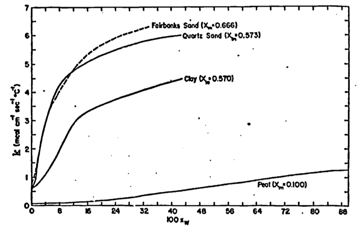
Figure 13.6: Dependence of the thermal conductivity k on the volume fraction of water \(X_W\) for four different soil types (from Sellers 1965)
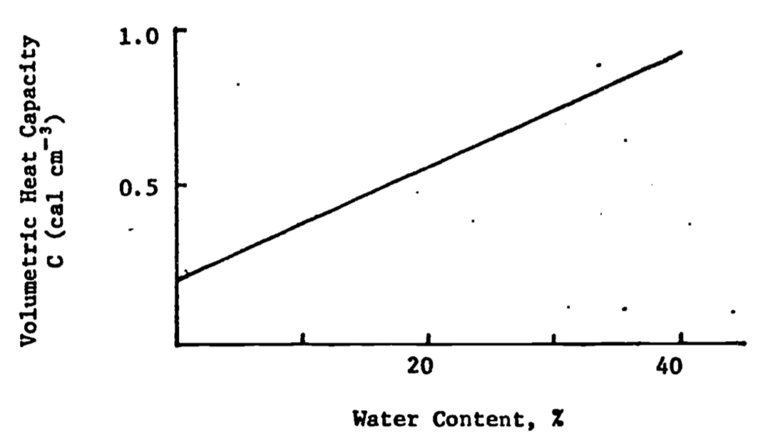
Figure 13.7: Variation of volumetric heat capacity (C) with water content in a typical soil (after Rose 1966)
13.4.2 Heat Storage and Energy Conservation
Equation (13.3) embodies the concept that heat flows from high to low temperature areas at a rate proportional to the temperature gradient. The constant of proportionality, \(k\), is a quantitative measure of a medium’s ability to transmit heat. As was discussed in the section on governing factors, complete specification of the temperature distribution also requires knowledge of the capacity of the medium to store heat for a given temperature change, i.e., its heat capacity. In general, heat capacity is defined on either a volumetric or mass basis. Specific heat capacity or specific heat (\(c\)) is defined in SI units as the amount of heat required to raise the temperature of 1 kg of material 1°C. Volumetric heat capacity is defined as \(C = \rho c\), where \(\rho\) is the density of the material. Table A (Appendix) lists dimensions and units of these quantities, while Table 13.1 lists typical values of specific heat for various materials. Taylor and Ashcroft (1972) present a more complete discussion from the viewpoint of thermodynamics.
The bulk heat capacity is generally estimated by adding up the heat capacities of the various soil constituents in a unit volume. The heat capacity per unit volume (\(C\)) can then be expressed as
\[\begin{equation} C=\rho c=X_mC_m+X_wC_w+X_aC_a+X_oC_o \tag{13.4} \end{equation}\]
where \(\rho\) is the soil density, \(X\) is volume fraction (dimensionless), and the subscripts \(m\), \(w\), \(a\), and \(o\) refer to minerals, water, air and organics, respectively (DeVries 1966). Use of Equation (13.4) is illustrated by DeVries (1966). Reliable experimental values of \(C_m\) , \(C_w\) , and \(C_o\) are (in cgs units) 0.46, 1.0, and 0.60 cal cm-3 °C-1. Calorimetric determination of the component heat capacities is discussed in detail by Taylor and Jackson (1965). \(C_a\) is small, and may be neglected, so that Equation (13.5) becomes
\[\begin{equation} C=0.46X_m+0.60X_o+X_w[cal\cdot cm^{-3}°C^{-1}] \tag{13.5} \end{equation}\]
It remains then to determine the volume fraction. Notice that for a given soil, \(X_m\) and \(X_o\) will be constant under our assumptions, but that \(X_w\) will change as the soil wets up or dries, making \(C\) a linear function of water content (Fig. 13.7). See DeVries (1966) for a more detailed discussion of heat capacity in soils.
Table 13.1. Thermal propertie8 of soils and their components (from Montieth, 1973).
| Water content \(x\delta\) | Density | Specific heat | Thermal conductivity | Thermal diffusivity | |
|---|---|---|---|---|---|
| \(\rho\) | \(c\) | \(k\) | \(K\) | ||
| tonne m-3(106 g m-3) | J g-1°C-1 | W m-1°C-1 | 10-6 m2 s-1 | ||
| (a) Soil components | |||||
| Quartz | 2.66 | 0.80 | 8.80 | 4.18 | |
| Clay minerals | 2.65 | 0.90 | 2.92 | 1.22 | |
| Organic matter | 1.30 | 1.92 | 0.25 | 1.00 | |
| Water | 1.00 | 4.18 | 0.57 | 0.14 | |
| Air (20°C) | 1.20 \(\times\) 10-3 | 1.01 | 0.025 | 2050 | |
| (b) Soils | |||||
| Sandy soil (40% pore space) | 0.0 | 1.60 | 0.80 | 0.30 | 0.24 |
| 0.2 | 1.80 | 1.18 | 1.80 | 0.85 | |
| 0.4 | 2.00 | 1.48 | 2.20 | 0.74 | |
| Clay soil (40% pore space) | 0.0 | 1.60 | 0.89 | 0.25 | 0.18 |
| 0.2 | 1.80 | 1.25 | 1.18 | 0.53 | |
| 0.4 | 2.00 | 1.55 | 1.58 | 0.51 | |
| Peat soil (80% pore space) | 0.0 | 0.30 | 1.92 | 0.06 | 0.10 |
| 0.4 | 0.70 | 3.30 | 0.29 | 0.13 | |
| 0.8 | 1.10 | 3.65 | 0.50 | 0.12 |
We are now in a position to write an equation for the conservation of energy, which by assumption 3 we limited to heat energy only. Assuming no work is done, the general form of this equation can be stated in words as \[\frac{\mbox{net flux of heat}}{\mbox{per unit volume and time}}=\frac{\mbox{rate of change of heat content}}{\mbox{per unit volume}}\] Assumption 3 in section 3 ruled out sources or sinks and conversion of heat energy into other forms. Consequently, if more heat is entering the volume of soil under consideration than is leaving, then the heat content (or more precisely internal energy), and thus the temperature, of the soil volume must be increasing as a function of time and vice versa.
Consider first a horizontal soil slab of thickness \(\Delta z\) and unit horizontal dimensions (Fig. 13.4). Recalling that in general \(G\) is a function of both depth and time, we let \(G(z,t)\) and \(G(z+\Delta z,t)\) be the heat flux density at the top and bottom of the slab, respectively, at the same instant of time \(t\). The difference \(G(z,t) - G(z+\Delta z,t)\) then represents the net heat storage in a slab of volume \(\Delta_z\) per unit of time and cross section. Using the definition of a partial derivative (see, e.g., Hildebrand 1962), and holding \(t\) constant, we may write this difference as the limiting expression
\[\begin{equation} \lim_{\Delta z\to0}[\frac{G(z,t)-G(z+\Delta z,t)}{\Delta z}]\Delta z=-\frac{\partial G}{\partial z}\Delta z \tag{13.6} \end{equation}\]
This amount of heat storage in the slab will cause a temperature change per unit of time \(\frac{\partial T}{\partial t}\). Assuming that the volumetric heat capacity \((C)\) is not a function of time, \(C\frac{\partial T}{\partial t}\Delta z\) represents the heat storage in a volume \(\Delta z\). This heat storage must be equal to that found in Equation 6 by consideration of differences in heat flux density. We may then write
\[C\frac{\partial T}{\partial t}\Delta z=\frac{\partial G}{\partial z}\Delta z\] Canceling out the common terms, we are left with an expression for the conservation of energy, \[\begin{equation} C\frac{\partial T}{\partial t}=-\frac{\partial G}{\partial z} \tag{13.7} \end{equation}\] This is also referred to as the continuity equation for heat transfer.
Notice the inclusion of a minus sign. The reason for this is illustrated by Fig. 13.4. If we consider the case when the soil volume is heating up, then \(C (\partial T/\partial t) > 0\). Now, for this to be the case, more heat must be entering the block \((G(z))\) than is leaving \((G(z+\Delta z))\), hence \(G(z,t) - G(z+\Delta z,t) > 0\), so \(\partial G/\partial z > 0\), by the definition of a partial derivative. Therefore, for Equation 13.7 to balance, the minus sign must be included. A similar argument holds when the soil is cooling.
13.4.3 Heat Conduction (Diffusion) Equation
Differentiation of the law of conduction (Equation 13.3) with respect to \(z\) and combining the result with the continuity equation (Equation 13.7) gives \[-\frac{\partial G}{\partial z}=\frac{\partial}{\partial z}(k\frac{\partial T}{\partial z})=C\frac{\partial T}{\partial t}\]
Again, invoking soil homogeneity with depth, we may write \[\begin{equation} \frac{\partial T}{\partial t}=K\frac{\partial^2T}{\partial z^2} \tag{13.8} \end{equation}\] where \(K = k/C = k/\rho c\) is called the thermal diffusivity. See Table 13.1 for units and some representative typical values of diffusivity. Equation (13.8) is commonly referred to as the diffusion equation. It arises in many physical and biological phenomena where the medium of interest can be considered homogeneous. Notice that while we have reduced our governing equation for heat flow to one dependent variable \((T)\), we retain the complexities inherent in equations containing partial derivatives. For further discussion of this type of equation, known as a partial differential equation, see e.g., Carrier and Pearson (1976).
The thermal diffusivity, \(K\), is an important parameter here for two reasons. First, it incorporates the thermal properties of the soil, \(C\) and \(k\), in one expression. The second is that its degree of functional dependence on \(t\), \(z\), or \(T\) will dictate the difficulty of the solution to Equation (13.8). In this latter regard, it is well to keep in mind that the simplified form of Equation (13.8) is due to our assumption that \(K\) is not a function of depth. To the extent that soil porosity and water content are functions of depth, application of Equation (13.8) is questionable. However, assumption of a constant thermal diffusivity, which we have alluded to before, will allow us to derive solutions to the problem illustrative of the general characteristics of soil heat flow.
The combination of \(k\) and \(C\) allows the one quantity \(K\) to determine the time necessary for the soil temperature to change in any situation. In Equation (13.8), we see that the change in temperature with time is related to the curvature of the temperature profile \((\partial^2 T/\partial x^2)\) through the diffusivity. The smaller the value of \(K\), for a given temperature profile, the longer it takes the soil to heat up, and vice versa. This is illustrated in Fig. 13.8, where an imaginary soil temperature gradient and its first and second derivatives are plotted. This figure also nicely demonstrates how one can deduce, simply from the temperature profile, what areas of the soil will be warming or cooling. Hence we have arrived at a quantitative justification for our reasoned speculation in section 2 that both \(k\) and \(C\) are essential for an adequate description of the soil temperature distribution.
Measurement of \(K\) and \(k\) are essentially the same, since they differ only by the quantity \(C\). In the section on Fourier’s law, we alluded to the difficulties encountered using steady state methods due to liquid or vapor transport of heat by soil water. Here we will briefly discuss transient methods (see e.g., Jackson and Taylor 1965, or Taylor and Ashcroft 1972). One is based on measurement of the heating and cooling rate of an electrically heated wire element in the soil. This rate is proportional to the diffusivity. Moisture movement during the heating cycle has been shown to be small for practical purposes. Another method is based on the solution of Equation (13.8) and actual temperature measurements in the field. This method’s accuracy is limited by the accuracy of our solution in terms of how well our assumptions fit the measurement site. More precise methods involving the direct measurement of \(G\) are discussed in Taylor and Ashcroft (1972). Dependence of \(K\) on soil water content is discussed in Rose (1966) and Sellers (1965).
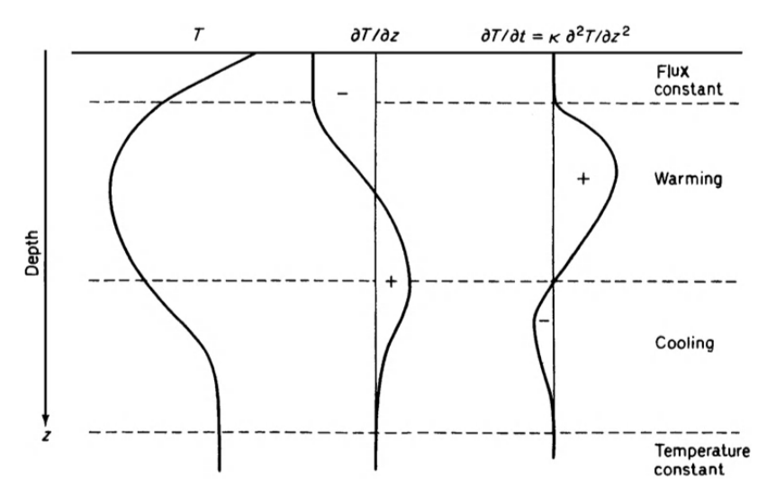
Figure 13.8: Imaginary temperature gradient in soil (left-hand curve), and the corresponding first and second differentials of temperature with respect to depth; i.e., \(\partial T/\partial z\) and \(\partial^2 T/\partial z^2\). The second differential is proportional to that rate of temperature change \(\partial T/\partial t\) (from Monteith 1973).
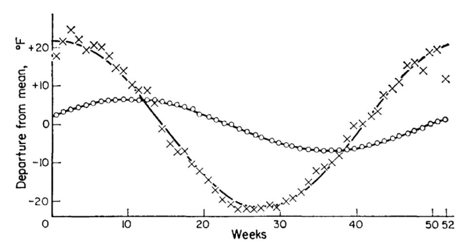
Figure 13.9: Record of the annual temperature wave at depths of 1m (X) and 2.5m (°) with fitted sine curves (from Rose 1966)