15.8 Sky Temperature
The sky temperature is the temperature you would measure if you pointed an infra-red thermometer at the sky. It is used to compute the downward flux of infra-red radiation and is estimated by the microclimate model as function of air temperature, cloud cover, relative humidity and shade.
The code below shows the values for each month and shade level at midnight. Note the extremely cold skies in central Australia in July in 0% shade, where the cloud cover and relative humidity are very low.
month<-1 # choose which month you want, 1 or 7 (i.e. Jan or Jun)
shade <- 0 # choose which month you want, 0 or 100%
Tsky_0shade_jan<-brick(paste0(path,"sky_temperature_degC/",shade,"_shade/TSKY_",
                              shade,"_",month,".nc")) # read the file into memory
shade <- 100 # choose which month you want, 0 or 100%
Tsky_100shade_jan<-brick(paste0(path,"sky_temperature_degC/",shade,"_shade/TSKY_",
                                shade,"_",month,".nc")) # read the file into memory
month<-7 # choose which month you want, 1 or 7 (i.e. Jan or Jun)
shade <- 0 # choose which month you want, 0 or 100%
Tsky_0shade_jul<-brick(paste0(path,"sky_temperature_degC/",shade,"_shade/TSKY_",
                              shade,"_",month,".nc")) # read the file into memory
shade <- 100 # choose which month you want, 0 or 100%
Tsky_100shade_jul<-brick(paste0(path,"sky_temperature_degC/",shade,"_shade/TSKY_",
                                shade,"_",month,".nc")) # read the file into memory

par(mfrow = c(2,2)) # set to plot 2 rows of 2 panels
plot(Tsky_0shade_jan[[1]],main = "Tsky 0% shade, 0:00 January, deg C", zlim = c(-20,20))
plot(Tsky_100shade_jan[[1]],main = "Tsky 100% shade, 0:00 January, deg C", zlim = c(-20,20))
plot(Tsky_0shade_jul[[1]],main = "Tsky 0% shade, 0:00 July, deg C", zlim = c(-20,20))
plot(Tsky_100shade_jul[[1]],main = "Tsky 100% shade, 0:00 July, deg C", zlim = c(-20,20))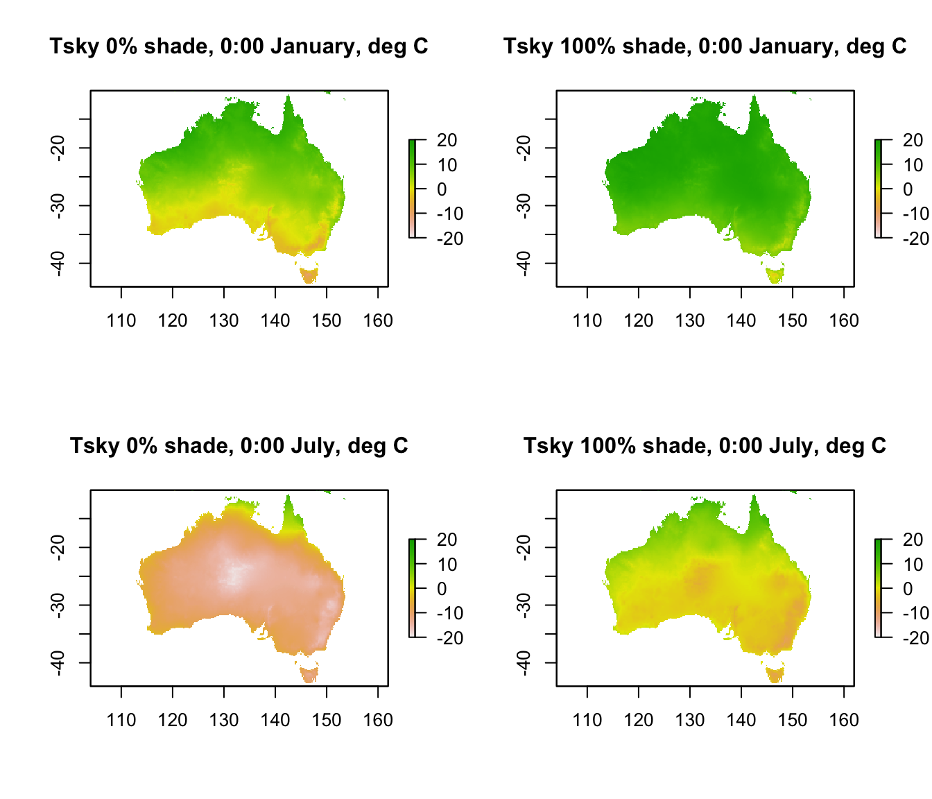
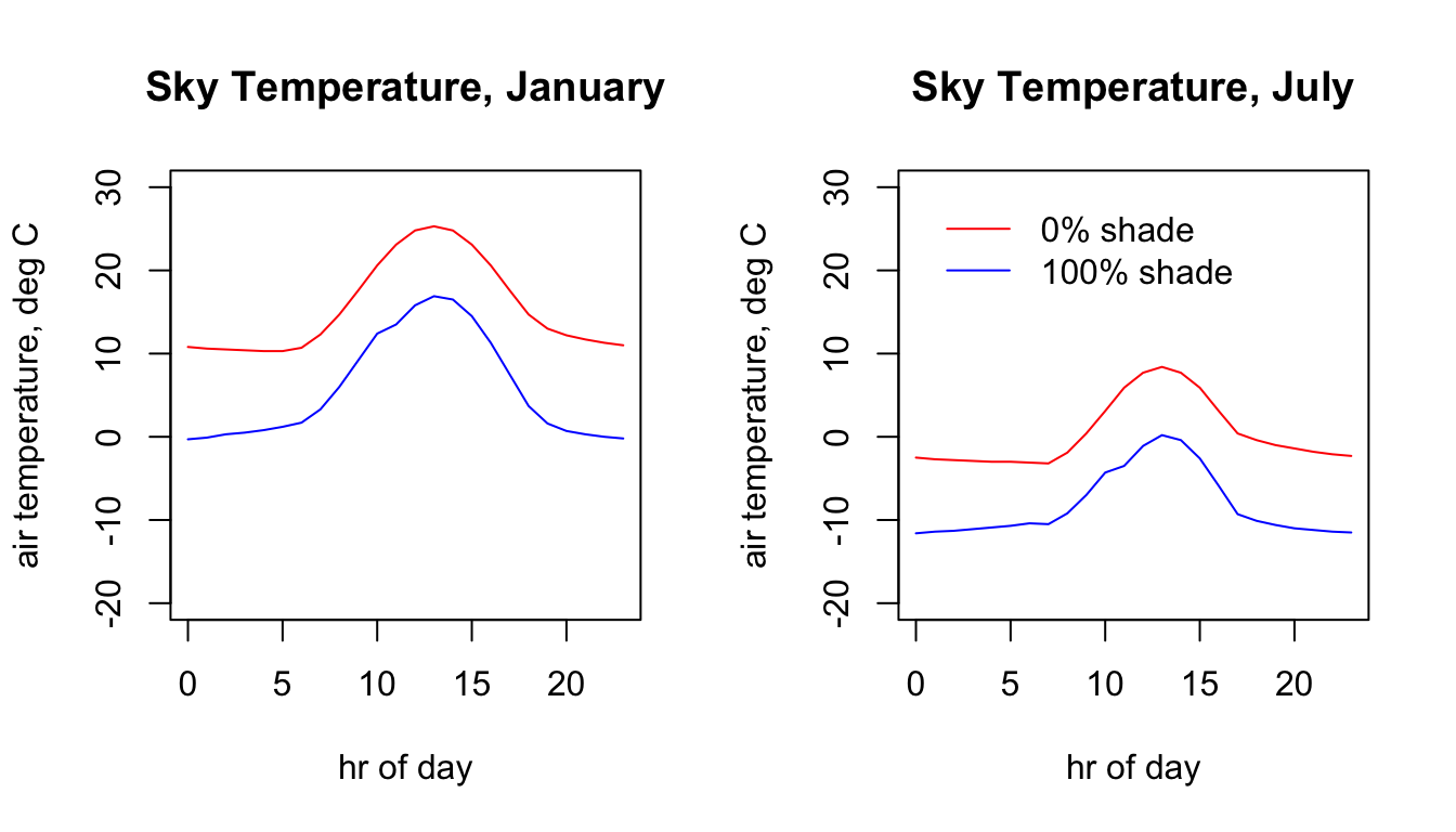
Here is the 24 hr pattern of sky temperature for the Flinders Ranges site each season for each shade level.
# extract data for all layers in 'Tsky_0shade_jan' at location 'lon.lat'
Tsky_0shade_jan.hr = t(extract(Tsky_0shade_jan, lon.lat))
# extract data for all layers in 'Tsky_0shade_jul' at location 'lon.lat'
Tsky_0shade_jul.hr = t(extract(Tsky_0shade_jul, lon.lat))
# extract data for all layers in 'Tsky_100shade_jan' at location 'lon.lat'
Tsky_100shade_jan.hr = t(extract(Tsky_100shade_jan, lon.lat))
# extract data for all layers in 'Tsky_100shade_jul' at location 'lon.lat'
Tsky_100shade_jul.hr = t(extract(Tsky_100shade_jul, lon.lat))

par(mfrow = c(1,2)) # set to plot 1 row of 2 panels
# plot sky temperature in 0% shade in January as a function of hour,
# as a line graph (using type = 'l'), in blue.
plot(Tsky_0shade_jan.hr ~ hrs, type = 'l', main = "Sky Temperature, January",
     ylab = "air temperature, deg C", xlab = "hr of day", col = 'blue', ylim = c(-20,30))
# plot sky temperature in 100% shade January as a function of hour,
# as a line graph (using type = 'l'), in red.
points(Tsky_100shade_jan.hr ~ hrs, type = 'l', col = 'red')

# plot sky temperature in 0% shade in July as a function of hour,
# as a line graph (using type = 'l'), in blue.
plot(Tsky_0shade_jul.hr ~ hrs, type = 'l', main = "Sky Temperature, July",
     ylab = "air temperature, deg C", xlab = "hr of day", col = 'blue', ylim = c(-20,30))
# plot sky temperature in 100% shade July as a function of hour, as a line graph (using type = 'l'),
# in red.
points(Tsky_100shade_jul.hr ~ hrs, type = 'l', col = 'red')

legend(0, 30, c("0% shade","100% shade"), col = c("red", "blue"), lty=c(1), bty = "n")