15.6 Wind Speed

For wind speed, notice how there are values for two heights, 1cm and 10m. The 10m value is what comes from the New et al. (2002) data set and is the height of the weather station wind speed measurements used by New et al. (2002) to interpolate the wind speed grids. But 10m isn’t a particularly useful height for calculating organismal heat and water budgets (well, except for trees and dinosaurs). The 1cm height was arbitrarily chosen as a useful general height at which to have microclimatic data, but this can be adjusted to different heights as discussed in Kearney et al. (2014).

The code chunk below reads in and plots the wind speed in January and July at midday at the two different heights.

month<-1 # choose which month you want, 1 or 7 (i.e. Jan or Jun)
# read the files into memory
V10m_jan<-brick(paste0(path,"wind_speed_ms_10m/V10m_",month,".nc")) 
V1cm_jan<-brick(paste0(path,"wind_speed_ms_1cm/V1cm_",month,".nc")) 
month<-7 # choose which month you want, 1 or 7 (i.e. Jan or Jun)
V10m_jul<-brick(paste0(path,"wind_speed_ms_10m/V10m_",month,".nc")) 
V1cm_jul<-brick(paste0(path,"wind_speed_ms_1cm/V1cm_",month,".nc")) 

par(mfrow = c(2,2)) # set to plot 2 rows of 2 panels
plot(V10m_jan[[13]],main = "wind speed 10m, 12:00 January, m/s", zlim = c(0,8))
plot(V1cm_jan[[13]],main = "wind speed 1cm, 12:00 January, m/s", zlim = c(0,2))
plot(V10m_jul[[13]],main = "wind speed 10m, 12:00 July, m/s", zlim = c(0,8))
plot(V1cm_jul[[13]],main = "wind speed 1cm, 12:00 July, m/s", zlim = c(0,2))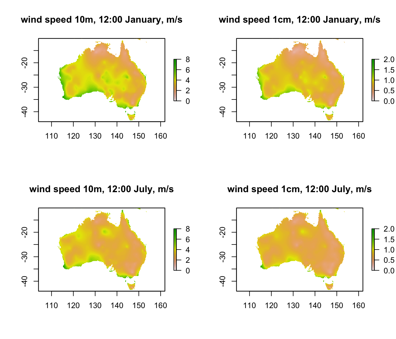

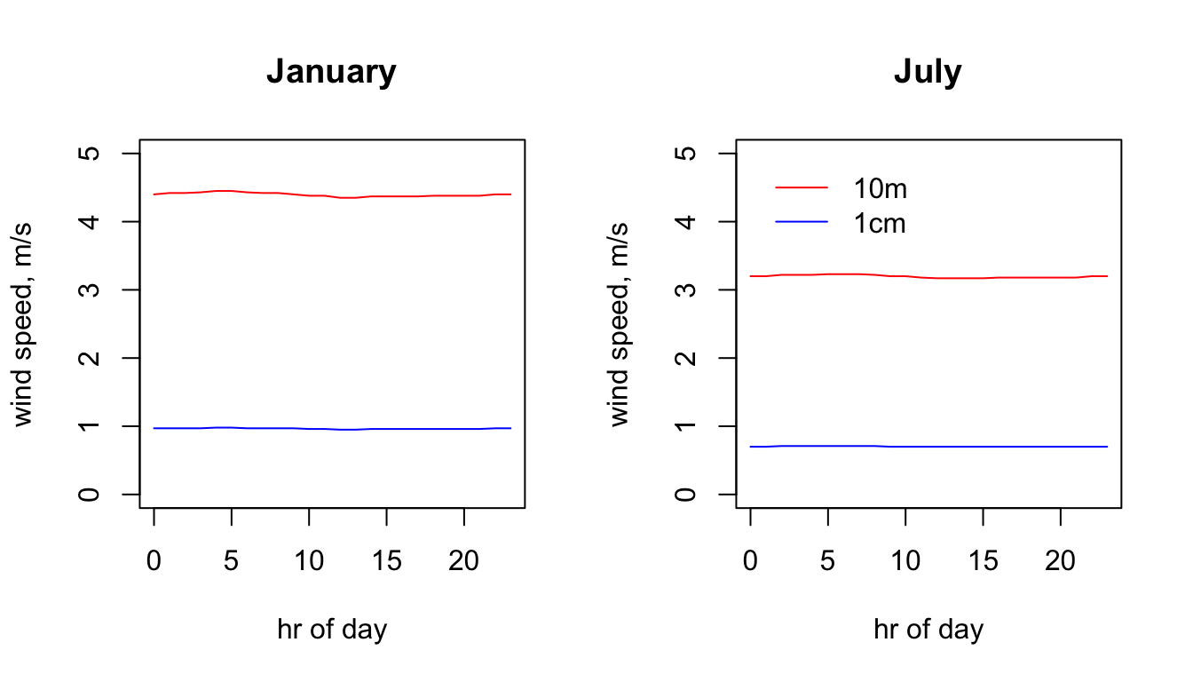
You can see that the coastal areas often have higher wind speeds, especially on the west coast in January. Note also the very big drop in wind speed as you go from 10m to 1cm (check the scale bars). The next code chunk plots the hourly wind speed at the Flinders Ranges site at each height in each month. Here, the magnitude of the difference between the heights is even clearer. Note also that there is no diurnal variation in wind speed in this data set because the New et al. (2002) data set does not have min/max wind speed but rather just the average daily wind speed.

# extract data for all layers in 'V10m_jan' at location 'lon.lat'
V10m_jan.hr = t(extract(V10m_jan, lon.lat)) 
# extract data for all layers in 'V10m_jan' at location 'lon.lat'
V1cm_jan.hr = t(extract(V1cm_jan, lon.lat)) 
# extract data for all layers in 'V1cm_jan' at location 'lon.lat'
V10m_jul.hr = t(extract(V10m_jul, lon.lat)) 
# extract data for all layers in 'V1cm_jan' at location 'lon.lat'
V1cm_jul.hr = t(extract(V1cm_jul, lon.lat)) 

# plot wind speed at 10m in January as a function of hour, as a line graph (using type = 'l'), in red
par(mfrow = c(1,2)) # set to plot 1 row of 2 panels
plot(V10m_jan.hr ~ hrs, type = 'l', main = "January", ylab = "wind speed, m/s", xlab = "hr of day", col = 'red', ylim = c(0,5)) 
# plot wind speed at 1cm in January as a function of hour, as a line graph (using type = 'l'), 
# with 10m in red and 1cm in blue.
points(V1cm_jan.hr ~ hrs, type = 'l', col = 'blue') 

# plot wind speed at 10m in January as a function of hour, as a line graph (using type = 'l'), in red
plot(V10m_jul.hr ~ hrs, type = 'l', main = "July", ylab = "wind speed, m/s", xlab = "hr of day", col = 'red', ylim = c(0,5)) 
# plot wind speed at 1cm in July as a function of hour, as a line graph (using type = 'l'), 
# with 10m in red and 1cm in blue.
points(V1cm_jul.hr ~ hrs, type = 'l', col = 'blue') 
 
legend(0, 5, c("10m", "1cm"), col = c("red", "blue"), lty=c(1), bty = "n")