11.7 Analysis of General Model
11.7.1 Calculations of Leaf Temperatures and Transpiration
It is straightforward to obtain values of the two dependent variables, leaf temperatures and transpiration rate, as a function of any conceivable combination of values of the independent variables and leaf parameters which appear in Equation (11.7). The four independent variables used are radiation absorbed, air temperature, relative humidity of the air, and wind speed; and the three leaf parameters are characteristic dimension, leaf width and internal resistance. Gates and Papian (1971) published a tabulation of leaf temperatures and transpiration rates for various sets of values of the dependent variables and leaf parameters. Similar plots are shown in a paper by Gates (1968). These plots have proved useful in understanding Equation (11.7), and therefore at this time we will undertake an explanation of how they are produced.
Let us begin by specifying \(Q_a = 800 W m^{-2}, T_a = 40°C, r.h. = 0.20, D = 0.05 m, W = 0.05 m, r_a = 0.0s m^{-1}\), and \(V = 0.10 m s^{-1}\). Now all the parameter values of Equation (11.7) are known except leaf temperature. We solve for leaf temperature and then calculate transpiration rate using the last term of equation (11.7). We examine the influence of varying wind speed and leaf resistance on transpiration as follows:
#radiation, convection, and evaporation
epsilon=0.96
#Stefan-Boltzmann's constant (W m^{-2}K^{-4})
sigma= 5.67 * 10^{-8}
#k1 is an experimentally determined coefficient ($9.14 J m^{-2} s^{-0.5} {^{\circ}C^{-1}}$)
k1=9.14
#k2 is an experimentally determined coefficient ($183 s^{0.5} m^{-1}$)
k2=200
#L, latent heat of vaporiation of water in J kg^{-1}, 2.43x10^6 at 30°C and 2.5*10^6 at 0°C
L=2.26*10^6

#calculate saturation vapor density
#' VAPPRS
#'
#' Calculates saturation vapour pressure for a given air temperature.
#' @param db Dry bulb temperature (°C)
#' @return esat Saturation vapour pressure (Pa)
#' @export
VAPPRS <- function(db=db){
  t=db+273.16
  loge=t
  loge[t<=273.16]=-9.09718*(273.16/t[t<=273.16]-1.)-3.56654*log10(273.16/t[t<=273.16])+
    .876793*(1.-t[t<=273.16]/273.16)+log10(6.1071)
  loge[t>273.16]=-7.90298*(373.16/t[t>273.16]-1.)+5.02808*log10(373.16/t[t>273.16])-
    1.3816E-07*(10.^(11.344*(1.-t[t>273.16]/373.16))-1.)+8.1328E-03*
    (10.^(-3.49149*(373.16/t[t>273.16]-1.))-1.)+log10(1013.246)
  esat=(10.^loge)*100
  return(esat)
}

#Solve vapour density
#rh: relative humidity, decimal%
#T: temperature, °C
#return Vapour density (kg m^{-3})
vd= function(T,rh){
rh=rh*100
  tk = T + 273.15
esat = VAPPRS(T)
e = esat * rh / 100
e * 0.018016 / (0.998 * 8.31434 * tk)
}

#____________
#Estimate T_l then estimate transpiration
est_TlTrans <- function(T_a=40, V=0.1, rh=0.2, r_l=0, D=0.05, W=0.05, Q_a=800) {
f<- function(T_l) epsilon *sigma*(T_l + 273)^4 + k1*(V/D)^0.5*(T_l-T_a) +
  L*(vd(T_l, rh)-rh*vd(T_a, rh))/(r_l + k2*(D^{0.3}*W^{0.20})/ V^{0.50})- Q_a
T_l=uniroot(f, interval=c(-100, 100))$root

#estimate transpiration
E=(vd(T_l, rh)-rh*vd(T_a, rh))/(r_l + k2*(D^{0.3}*W^{0.20})/ V^{0.50})
return(c(T_l, E))
}
#----

#Vary V
par(mar = c(5, 5, 3, 5))
fig2a=sapply( seq(0.1,6.1,0.2), FUN=est_TlTrans, T_a=40, rh=0.2,
              r_l=0, D=0.05,
              W=0.05, Q_a=800)
plot(fig2a[1,], fig2a[2,], type="l", xlab="Leaf temperature (°C)",
     ylab= expression("Leaf transpiration (kg / " * m^2 * "s)"))

#Vary r_l
fig2b=sapply( seq(0,600,10), FUN=est_TlTrans, T_a=40, V=2.1, rh=0.2,
              D=0.05, W=0.05, Q_a=800)
points(fig2b[1,], fig2b[2,], type="l", col="red")

legend("topright", c("Vary windspeed", "Vary leaf resistance"),
       col = c("black", "red"), lty=c(1), bty = "n")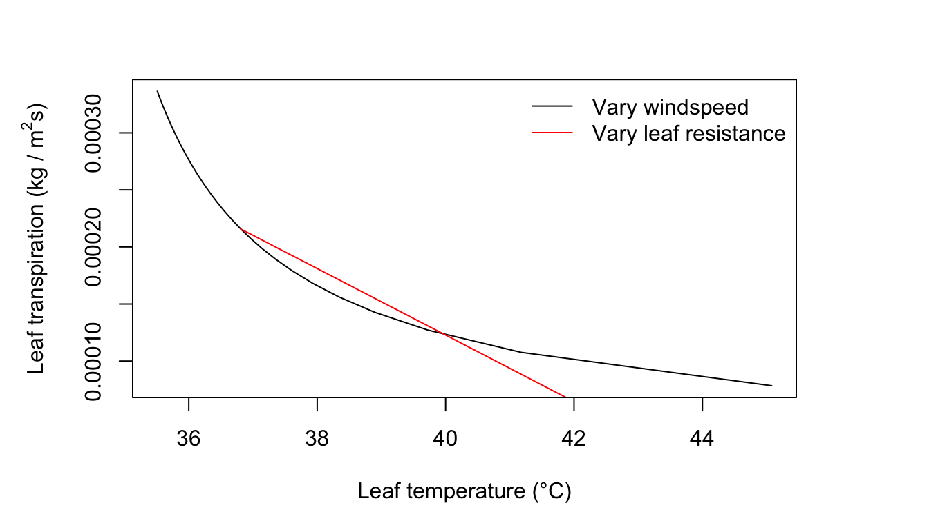
Figure 11.2: Leaf transpiration verses leaf temperature.
11.7.2 Sample Plots of Transpiration and Leaf Temperature
It is possible to select as changing variables in the graph any two of the following independent variables and leaf parameters: amount of radiation absorbed, air temperature, wind speed, relative humidity, leaf dimensions, and diffusion resistance. For our first example, we shall use, as changing variables, wind speed and internal diffusion resistance. Let wind speed values be 0.1, 2.1, 4.1, and 6.1 ms-1, and internal diffusion resistance values be 0, 200, 400, and 600 sm-1.
A leaf size of \(0.05 \times 0.05 m\) is selected for the first examples. Plots are generated for the following conditions:
- \(Q_a = 800 W m^{-2}; T_a = 40^\circ C; r.h. = 0.20\)
- \(Q_a = 700 W m^{-2}; T_a = 30^\circ C; r.h. = 0.20\)
- \(Q_a = 700 W m^{-2}; T_a = 30^\circ C; r.h. = 0.80\)
- \(Q_a = 300 W m^{-2}; T_a = 10^\circ C; r.h. = 0.50\)
We create the plots in R:
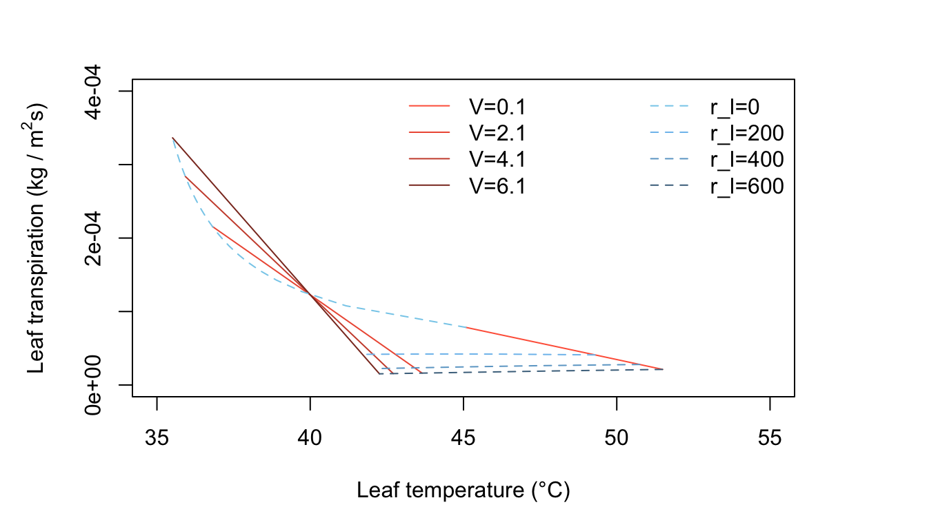
Figure 11.3: Leaf transpiration versus leaf temperature.
Figure 11.3 has many interesting features. It is characteristic of a hot, dry, high intensity radiation environment, such as one finds in a desert. In still air, represented by \(V = 0.1 m s^{-1}\), a leaf with a high diffusion resistance becomes very warm. For \(r_l = 600 s m^{-1}, T_l = 45°C\), but if \(r_l = \infty\), \(T_l\), is nearly \(15^\circ C\) above the air temperature of \(40^\circ C\). This can only be obtained by extrapolating the straight line for \(V = 0.1 m s^{-1}\) to where it intersects the temperature axis at zero transpiration. It is evident that all the constant wind speed lines intersect and cross over at \(T_l=T_a= 40^\circ C\). Note the small decrease in transpiration rate for \(r_l = 600 s m^{-1}\) when \(T < 42^\circ C\) and the wind speed has increased to \(V = 2.1, 4.1,\) and \(6.1 m s^{-1}\). This is an interesting phenomenon and should be understood by the reader. Look at Equation (11.7) and consider the effect of increased wind speed. An increase of \(V\), when the leaf temperature is above the air temperature, produces a decrease of leaf temperature by convective cooling. The increased wind speed also diminishes the thickness and resistance of the leaf boundary layer. This, by itself, would cause the transpiration rate to increase. However, the convective cooling of the leaf caused the water vapor pressure inside the leaf to drop and that produces a reduction of transpiration. In effect, what happens is that there is a greater reduction of the numerator in the evaporation term of Equation (11.7) (the driving force) than there is of the denominator (the resistive force). This phenomenon shows up at relatively high values of internal leaf resistance. At lower leaf resistance values, of \(400 s m^{-1}\), when the wind speed increases the transpiration rate increases and the line of constant internal leaf resistance turns upward with wind speeds greater than about \(1 m s^{-1}\) (see Figure 11.3, line 3).
Now consider what happens when the leaf diffusion resistance is small, e.g., \(200 sm^{-2}\). Here in Figure 11.3, the line at constant \(r_l = 200 s m^{-1}\) is doubled valued in \(E\) for certain \(T_l\). The line curves back on itself as wind speed increases. At first, as the wind speed increases from \(0.1 m s^{-1}\) to about \(1.0 m s^{-1}\), the leaf temperature decreases as the transpiration rate increases, but at higher wind speeds; although the transpiration rate continues to increase, the leaf temperature begins to increase. At very high wind speeds, it would approach the air temperature because convection is transferring heat to the leaf since the air is warmer than the leaf. A general feature of Figure 11.3 is that for hot, dry, high radiation conditions, a leaf is warmer than the air temperature if the internal diffusion resistance is above a certain value– here, estimated at about \(300 s m^{-1}\). If the leaf resistance is less than this value, the leaf temperature is below the air temperature.
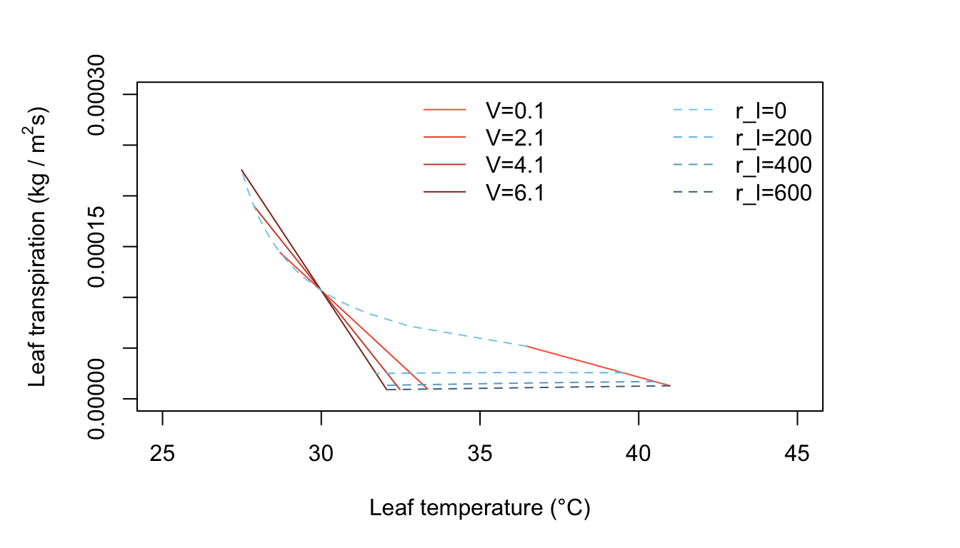
Figure 11.4: Leaf transpiration versus leaf temperature.
Figure 11.4 represents leaf temperature and transpiration rates for warm, dry, moderate radiation conditions, with \(V\) and \(r_l\) as changing quantities. Only leaves with relatively low internal resistance have temperature less than the air temperature. Leaves with resistances of about \(200 s m^{-1}\) or greater will be from 0 to about 8°C above air temperature, depending on the wind speed (Figure 11.4). Where does the line of zero internal diffusion resistance show up in this figure or is it beyond the scale used?
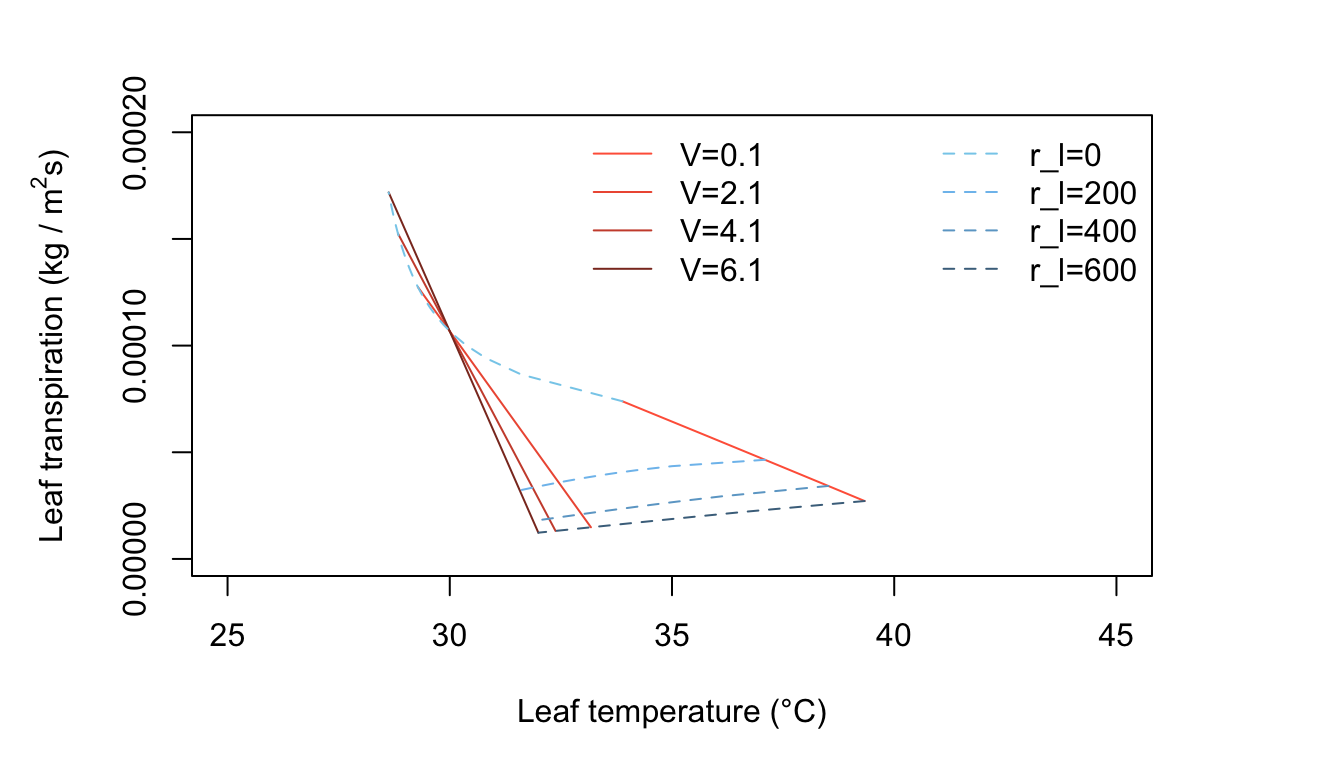
Figure 11.5: Leaf transpiration versus leaf temperature.
Figure 11.5 is for warm, humid, moderate radiation intensity conditions such as occur in many tropical situations and during moist, summer temperate region days. Transpiration rates are generally low, since the vapor density difference between leaf and air is not very great. Now the leaf temperatures are always above the air temperature for all realistic values of \(r_l\).
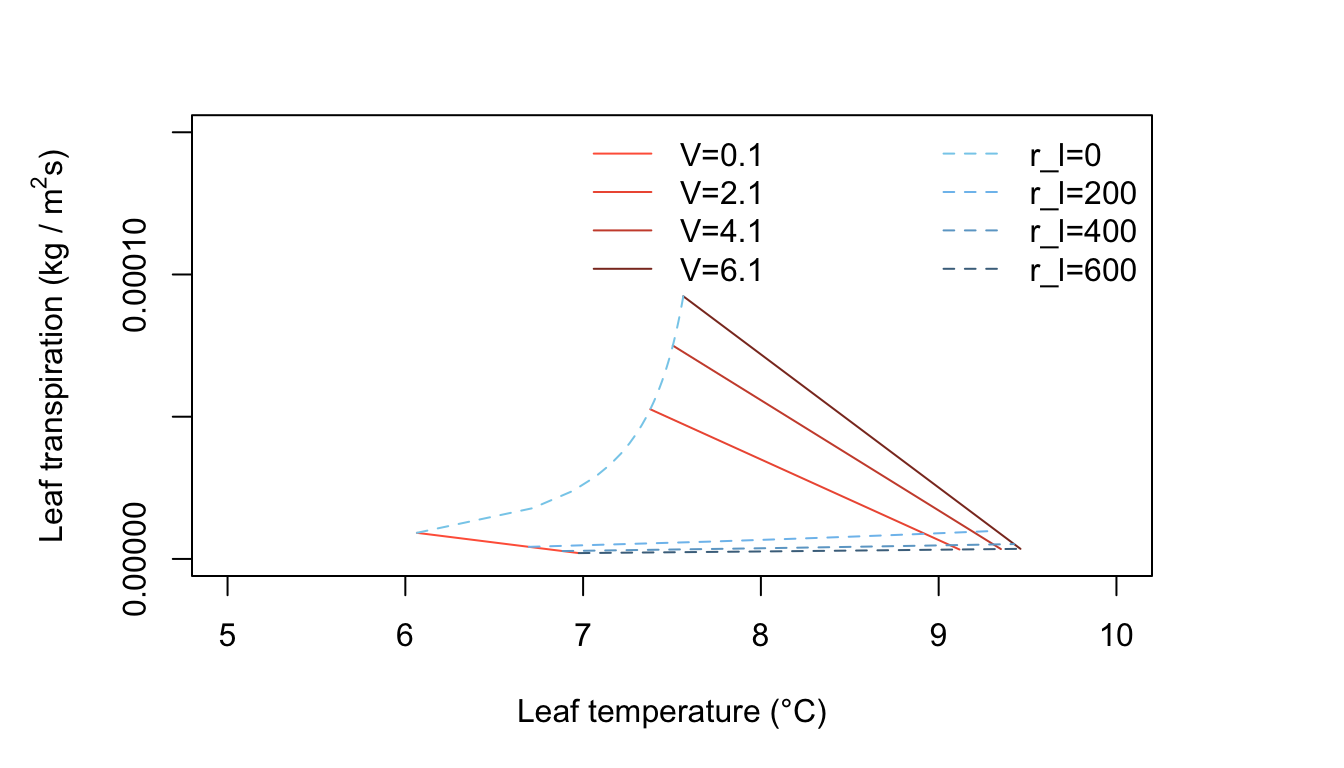
Figure 11.6: Leaf transpiration versus leaf temperature.
Figure 11.6 represents cool, moderately humid, low radiation conditions and exhibits some interesting features. All leaf temperatures are below the air temperature. An increase of wind speed always warms the leaf and, at constant internal leaf resistance, produces a small increase of transpiration. Generally, the transpiration rates are very low because of the limited amounts of energy available. The line of zero leaf resistance constant is well displayed here. The reader should ask if the conditions used here, e.g., \(Q_a = 300 W m^{-2}, T_a = 10^\circ C,\) and \(r.h, = 0.50\) are realistic and, if so, when and where will they occur.
Now it is possible to explore other dimensions of the transpiration-leaf temperature plot. Let the changing variables be air temperature and internal diffusion resistance. Use air temperature of 10, 20, 30, and 40°C and resistance of 0, 333, 667, and 1000 \(s m^{-1}\). The leaf size is \(0.05 \times 0.05 m\) as before. Plots are generated for the following conditions:
- \(Q_a = 700 W m^{-2}; V = 0.1 ms^{-1}; r.h. = 0.20\)
- \(Q_a = 700 W m^{-2}; V = 0.1 ms^{-1}; r.h. = 0.80\)
- \(Q_a = 700 W m^{-2};V = 2.0 ms^{-1}; r.h. = 0.50\)
- \(Q_a = 700 W m^{-2}; V = 0.1 ms^{-1}; r.h. = 0.50\)
We create the plots in R:
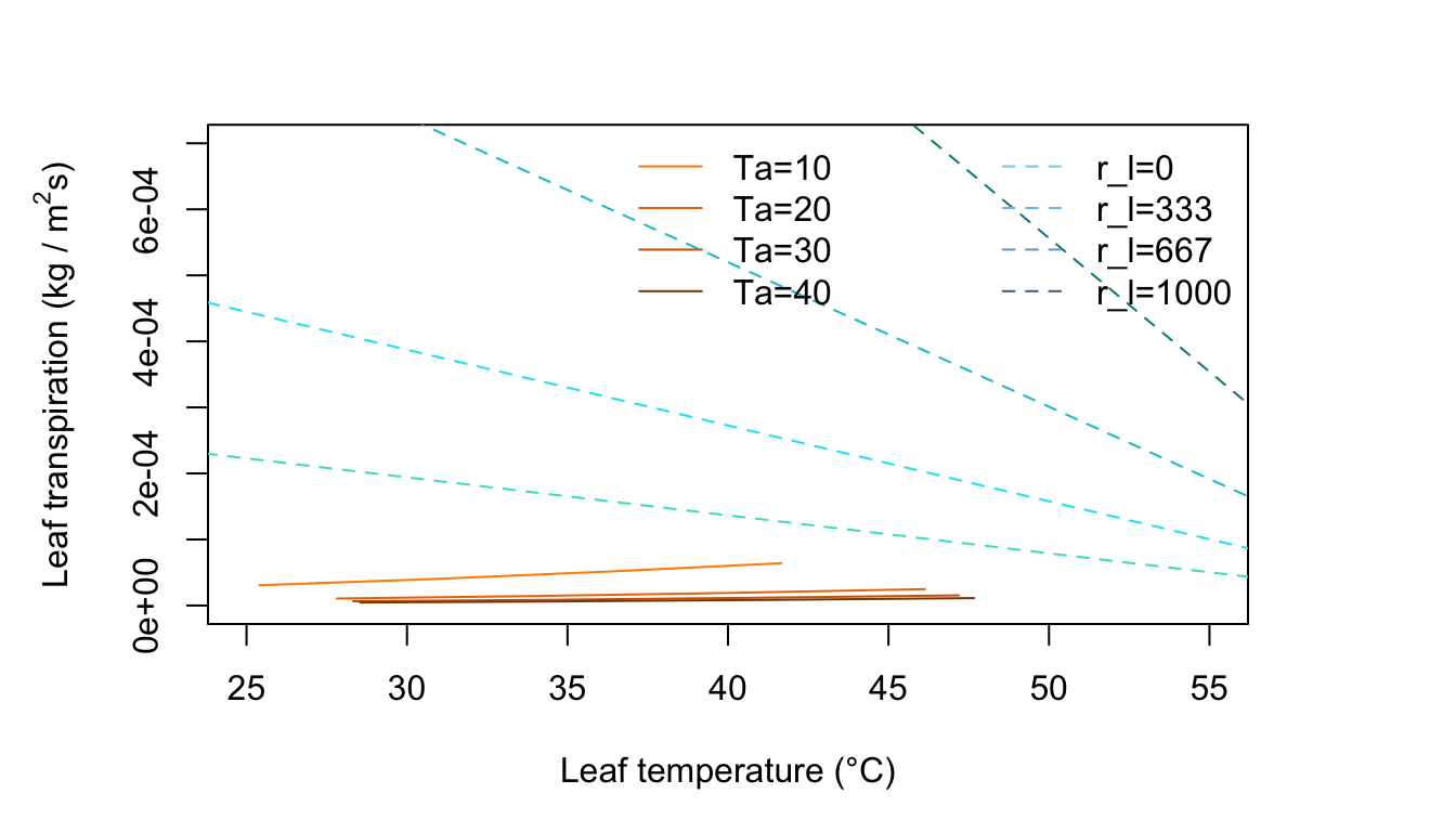
Figure 11.7: Leaf transpiration versus leaf temperature.
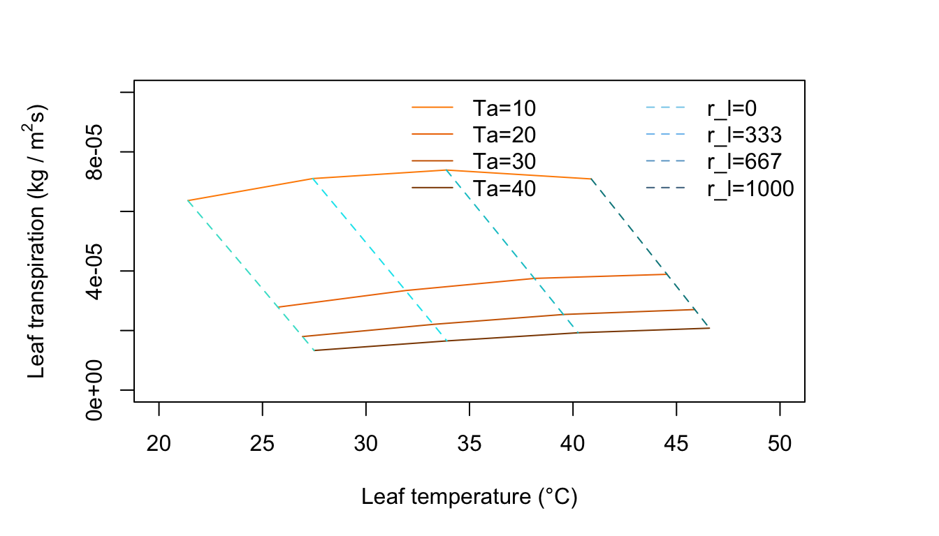
Figure 11.8: Leaf transpiration versus leaf temperature.
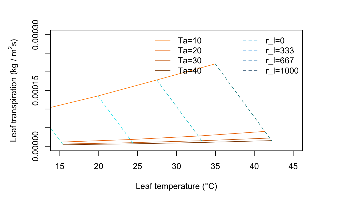
Figure 11.9: Leaf transpiration versus leaf temperature.
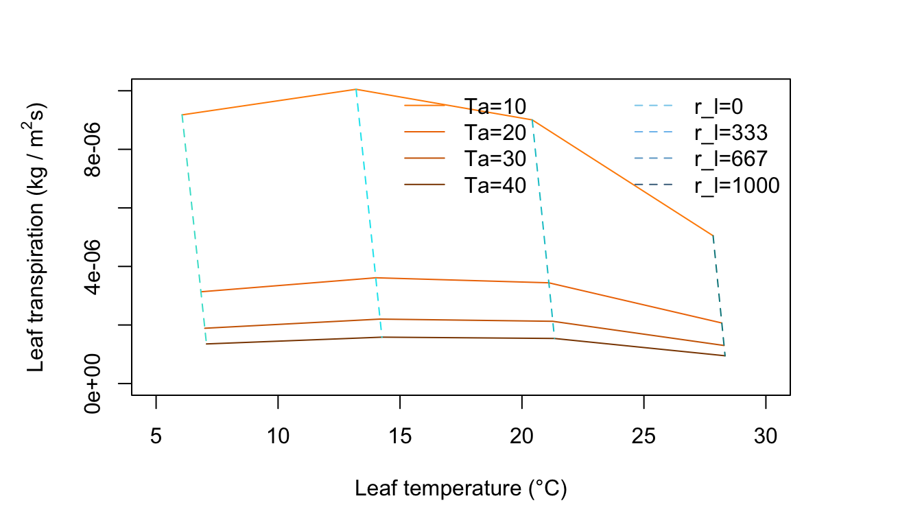
Figure 11.10: Leaf transpiration versus leaf temperature.
Figure 11.7 represents an environment of no wind, moderate radiation intensity, and very dry air. There are lines of constant air temperature. Note where it is in the plot that \(T_l > T_a\) and \(T_l < T_a\) . Locate the transition point on the air temperature lines and draw a light line connecting these.
Figure 11.8 is for an environment of no wind, moderate radiation intensity and high humidity. Compare this with Figure 11.7. Notice the change in slope of the constant temperature lines and the curvature of the constant resistance lines. There is an optimum temperature for the freely evaporating surface with zero internal resistance. Why? As the air temperature increase from 10 to 20 to 30°C along a constant resistance line, the leaf temperature is increasing but at the same time the difference \(T_l - T_a\) is getting smaller. Since the term for radiation emitted by the leaf increases with the fourth power of \(T_l\), it is taking up a disproportionate amount of the available energy which is constant at \(Q_a = 700 W m^{-2}\), Not only is there less energy available for convection, but less for evaporation of water. Also, as \(T_a\) increases, the vapor density difference in the evaporation term of Equation (11.7) becomes less and the driving force to remove moisture from the leaf diminishes.
Figure 11.9 is for conditions of moderate radiation intensity, moderate humidity, and light wind. The rate of transpiration has increased over that in Figures 11.7 and 11.8. Here the leaf temperature is above air temperature for high resistance values, but for low resistances it is below; whereas in Figure 11.8, it was above air temperature for nearly all of the graph.
Figure 11.10 is for a low amount of absorbed radiation, no wind, and moderate humidity. The constant air temperature lines are very steep and the leaf temperature is always less than the air temperature. Note that for each constant resistance line, there is an optimum air temperature for which transpiration is a maximum. Why does transpiration diminish at high air temperatures? Are the environmental conditions realistic throughout the graph? Is the amount of radiation absorbed by the leaf consistent with the air temperature regime throughout the plot? If not, draw a line on the graph demarking a region of real environments from unreal ones.