6.3 Applications of the First Law

When thinking of the ecological implications of work for an organism one might imagine an animal moving or a plant transporting fluid. In these cases chemical energy is used to do mechanical work. In accord with the Second Law of Thermodynamics, these are not 100 percent efficient processes and heat is thus liberated.

Heat is usually a negligible component of the energy balance of plants. Interesting exceptions to this general statement are several species of the Araceae family including skunk cabbage, Lysichitum americanum; the water lily, Victoria; and arum lilies, Arum italicum (Fisher 1960, Meeuse 1975).

6.3.1 Work

In contrast, we know from our own experience that during physical exercise we can generate a large amount of heat because of our increased metabolic rate (necessary to do the mechanical work associated with the exercise). While jogging in place or skipping rope there may be no increase of potential energy (such as when climbing a hill) but work is performed by accelerating and decelerating the legs and arms. How the mechanical work is related to increased metabolic rate is currently a topic of interest for comparative physiologists studying locomotion (Bartholomew 1977, Taylor et al. 1970). For our purposes, the metabolic rate can be measured directly and included in the heat energy balance of organisms. To illustrate the case in which $Q = 0$ and work is non-zero, we present a meteorological example that is of interest to the ecologist.

The following example can be found in many introductory micrometeorology texts as well as in MacArthur (1972). It is a well-known fact that air cools as it rises. It is especially evident and ecologically important as one goes up the side of a mountain. Not only does the temperature fall but usually moisture is released. The reason for this phenomenon is that at higher elevations the atmosphere is less dense, so that as a unit of air (the system) rises, it pushes out, thus doing work and changing its internal energy. Therefore we define the system as a parcel of air, while surrounding it is the atmosphere enclosing the parcel.

What we would like is an expression to relate the change in height to the change in temperature. The physical law needed is the First Law of Thermodynamics with no heat flux ($Q = 0$, adiabatic process). We have then \[\begin{equation} dU = -W \tag{6.2} \end{equation}\]

In the module developing the theory of the First Law we also developed two other relationships in the piston example. One is that the change in internal energy $dU$ is equal to the heat capacity $C_V$ times the change in temperature $dT$ (for a reversible process revolving an ideal gas). \[\begin{equation} dU = C_V dT \tag{6.3} \end{equation}\] Secondly we discovered that the work $W$ done by the system on the surroundings is equal to $P dV$ so \[\begin{equation} W = P dV \tag{6.4} \end{equation}\] By substituting equations (6.3) and (6.4) into equation (6.2) we express the First Law as \[\begin{equation} C_V dT = -P dV \tag{6.5} \end{equation}\] Furthermore, we know that the state variables are related by the Ideal Gas Law $P V = R T$ which in total differential form is \[\begin{equation} V dP +P dV = R dT \tag{6.6} \end{equation}\] Since our goal is to express the temperature change as a function of height or elevation we will eliminate $P dV$ from equation (6.5) by substituting into equation (6.6) which yields \[\begin{equation} C_V dT = -R dT + V dP \tag{6.7} \end{equation}\] The rationale for this step is based on the fact that we can define the change in pressure with the change in altitude. This relation is derived by considering a parcel of air.

If we assume a unit cross section, then the change of pressure is equal to the unit weight $w$ of air at height $h$ times the change in height \[\begin{equation} dP = -w\:dh \tag{6.8} \end{equation}\] Furthermore \[\begin{equation} w = g \frac{m}{V} \tag{6.9} \end{equation}\] where

$g$ is the acceleration of gravity,
$m$ is molecular mass of air,
and $V$ is the volume of one mole.

Combining equations (6.8) and (6.9) and rearranging we have \[\begin{equation} V dP = -g m dh \tag{6.10} \end{equation}\]

Substituting equation (6.10) into (6.7) and rearranging we have $(c_V + R) dT = -g m d$ the desired result; a formula that tells us how temperature changes with height. (Also recall that for an ideal diatomic gas that the heat capacity at constant volume $C_V = 2.5 R.$) \[ \frac{dT}{dh} = \frac{-g\,m}{C_V + R} = \frac{-9.8ms^{-2} \cdot 0.029 kg mole^{-1}}{8.314 J {^{\circ}C}^{-1} (2.5+1) J {^{\circ}C}^{-1} mole^{-1}} = 0.0098 \frac{^{\circ}C}{m} = -9.8 \frac{^{\circ}C}{km}\]

Thus the air temperature will be $10 ^{\circ}C$ lower for each kilometer increase in altitude. This is called the adiabatic lapse rate (no external source of heat). In many locations the rising air contains moisture, which condenses as the air rises thus adding the heat of condensation to the dry adiabatic lapse rate. Therefore the “moist adiabatic” lapse rate of about $6 \frac{^{\circ}C}{km}$ is less than the dry adiabatic lapse rate. Interestingly enough the reverse effect, air moving down a mountain, also occurs. These winds are known as foehn winds in the Alps and the Chinook winds in the Rocky Mountains. As the winds come down the leeward side of the mountain the atmospheric pressure increases causing as much as a 15-20 $^{\circ}C$ rise in temperature.

6.3.2 Examples of Heat Energy Exchange

The next set of examples is used to illustrate the First Law for systems in which it can be assumed that the work term is zero. Therefore \[\begin{equation} \Delta U = Q \tag{6.11} \end{equation}\]

Any change in the internal energy of the system as measured by a change in temperature is due to heat flow. The general heat balance equation is \[\begin{equation} \Delta U = Q_a + M + P - Q_e - LE - G - C \tag{6.12} \end{equation}\] where

$\Delta U$ = change in internal energy ($W m^2$, watts per square meter),
$Q_a$ = radiation absorbed by the system surface($W m^{-2}$),
$P$ = photosynthesis ($W m^{-2}$),
$M$ = basal metabolism($W m^{-2}$),
$Q_e$ = radiation emitted by the system surface ($W m^{-2}$),
$L$ = latent heat of evaporation ($J kg^{-1}$),
$E$ = evaporation flux density ($kg m^2 s^{-1}$),
$G$ = conduction ($W m^{-2}$),
and $C$ = convection ($W m^{-2}$).

Equation (6.12) is a general heat flow equation. In most cases except for water vapor flux $LE$, mass exchange can be neglected. Similarly, the system’s internal sources of heat energy, photosynthesis and metabolism, are also very small components of the heat energy budget and can usually be ignored. We note, however, there are important exceptions of which the largest group includes endothermic vertebrates, birds and mammals. The other terms $Q_a$, $Q_e$, $LE$, $C$, $G$ of equation (6.12) represent the basic heat transfer processes that were described in the first module entitled “The First Law of Thermodynamics for Ecosystems.”

The first example we wish to consider is the heat energy budget of the earth. For the simplicity of the following example, we will for the moment put asie anthropogenic global warming, and assume the average temperature of both the earth and the atmosphere are not changing with time. Thus, we assume $\Delta U = 0$. Therefore the sum of the heat fluxes is zero and \[\begin{equation} 0 = Q_a - Q_e -LE -C \tag{6.13} \end{equation}\] where

$Q_a$ = radiation absorbed from the sun (left half of Fig. 6.2),
$Q_e$ = energy emitted by the atmosphere and earth,
$LE$ = heat loss by evaporation or latent heat,
and $C$ = convection or sensible heat.

Now consider figure 6.1 where the numbers represent the percentage of the total energy from the sun. If we define the earth and atmosphere as the system and space as the surroundings, the sum of the heat fluxes should be zero across the system’s boundary. Checking the numbers, we receive 100 percent and lose 25, 9, 48 and 18 percent which adds to a net flux of zero. Likewise we can take the earth as the system. Also notice what happens to the direct solar radiation as it enters the atmosphere. Only 47 percent reaches the ground level. The atmosphere acts as a trap. It absorbs the short wave radiation and reradiates longwave radiation. Furthermore, about 23 percent of the available heat energy from the sun is used in evapotranspiration. This process reduces air temperature in wet climates and redistributes moisture.

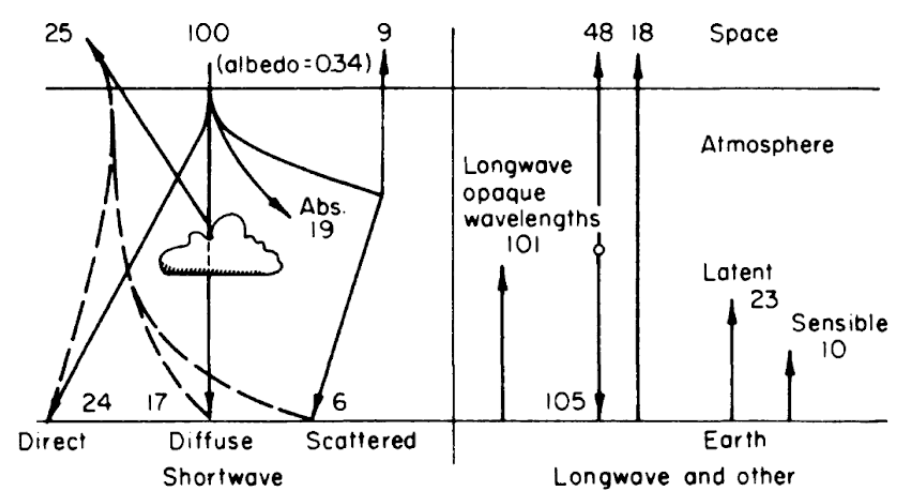
Figure 6.1: Relative net transfer of heat within the earth-atmosphere-space system. From Lowry, W.P. 1969. P. 27.

Our next example is that of a small stream taken from Brown (1969). Fish and game managers noted that clear cutting to the water’s edge eliminated trout and salmon populations. Brown modeled the energy exchange to determine how manipulation of streamside vegetation could reduce large diurnal fluctuations and high water temperatures, a potential cause of mortality. Again the First Law is used to say that the change in internal energy is equal to the sum of the heat flows. \[\begin{equation} \Delta U = + Q_{NR} - LE - G - C \tag{6.14} \end{equation}\] where

$\Delta U$ = net change in internal energy of the stream ($W m^{-2}$),
$Q_{NR}$= net thermal radiation flux ($Q_a - Q_e$)($W m^{-2}$),
$LE$ = evaporative flux ($W m^{-2}$),
$G$ = conductive flux ($W m^{-2}$),
and $C$ = convective flux ($W m^{-2}$).

Brown measured the heat fluxes of three different systems: 1) a forested section, 2) a nonforested gravel bottom section, and 3) a nonforested rockbottom section. Changes in water temperature were computed hourly using the fact that $\Delta T = \Delta U$ divided by heat capacity where the heat capacity is equal to the surface area of the water divided by the flow rate times the specific heat of water. In Part a of Figs. 6.2 through 6.4 Brown used the energy fluxes to calculate $\Delta U$. From these values $\Delta T$ is calculated and added to the water temperature at the beginning of the stream section to get the predicted water temperatures shown in part b of each figure.

In Fig. 6.2a the energy components of equation (6.14) are plotted as a function of time of day for a section of the stream covered by the forest. The water temperature at the end of the reach can be predicted as described above. In Fig. 6.2b the observed and predicted temperatures at the end of the section are compared. Since net radiation is small because the section is forested there is not much change in temperature throughout the day.

In Figs. 6.3a and 6.3b similar graphs illustrate the results Brown got for a nonforested gravel bottom section. Net radiation is the largest term of the energy budget and causes a large increase in water temperature.

The values depicted in Figs. 6.4a and 6.4b are for a site which also was unforested. Unlike the previous example where the bed of the stream was gravel and conduction was small, this site had a solid rock bottom and here heat passed from the stream into the stream bed, indicating a substantial conduction component of the energy balance.

Generally the results indicate that the model is very successful in predicting water temperature. The evaporation and convection fluxes are small at all sites. Net radiation is the major component of the heat balance of which the major factor is direct solar radiation. This is especially true for the nonforested sites (Figs. 6.3a and 6.4a). It is also interesting to note that conduction is an important component of the heat balance for the rocky-bottomed streambed (Fig. 6.4a) but not the gravel bottom (Fig. 6.3a).

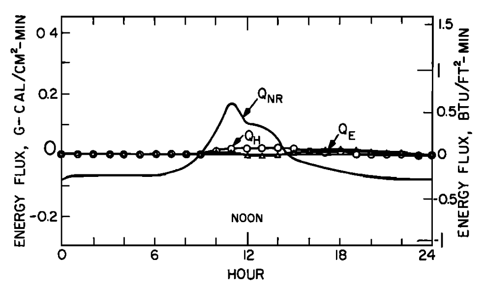
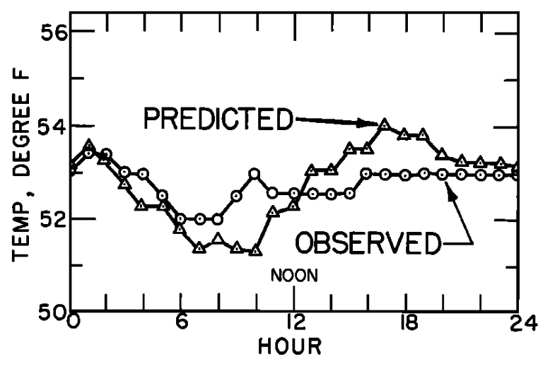
$a) The daily pattern in net thermal radiation ($Q_{NR}$), evaporation ($Q_E$), and convection ($Q_H$) for the forested Deer Creek study section. From Brown, G. W. 1969: P. 71,72. b) Observed and predicted hourly temperature for the forested Deer Creek study section. From Brown, G. W. 1969. P. 71,72.$ $a) The daily pattern in net thermal radiation ($Q_{NR}$), evaporation ($Q_E$), and convection ($Q_H$) for the forested Deer Creek study section. From Brown, G. W. 1969: P. 71,72. b) Observed and predicted hourly temperature for the forested Deer Creek study section. From Brown, G. W. 1969. P. 71,72.$

Figure 6.2: a) The daily pattern in net thermal radiation ($Q_{NR}$), evaporation ($Q_E$), and convection ($Q_H$) for the forested Deer Creek study section. From Brown, G. W. 1969: P. 71,72. b) Observed and predicted hourly temperature for the forested Deer Creek study section. From Brown, G. W. 1969. P. 71,72.

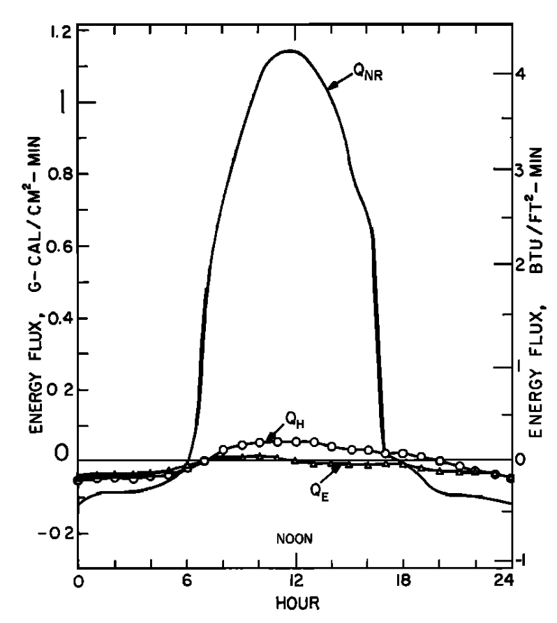
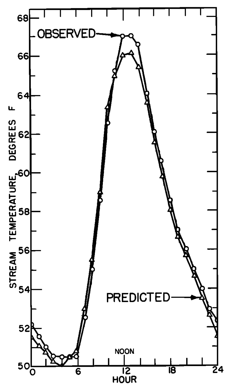
$a) The daily pattern in net thermal radiation ($Q_{NR}$), evaporation ($Q_E$), and convection ($Q_H$) for the nonforested gravel bottom Berry Creek study section. From Brown, G. W. 1969: P. 72. b) Observed and predicted hourly temperature for the nonforested gravel bottom Berry Creek study section. From Brown, G. W. 1969. P. 72.$ $a) The daily pattern in net thermal radiation ($Q_{NR}$), evaporation ($Q_E$), and convection ($Q_H$) for the nonforested gravel bottom Berry Creek study section. From Brown, G. W. 1969: P. 72. b) Observed and predicted hourly temperature for the nonforested gravel bottom Berry Creek study section. From Brown, G. W. 1969. P. 72.$

Figure 6.3: a) The daily pattern in net thermal radiation ($Q_{NR}$), evaporation ($Q_E$), and convection ($Q_H$) for the nonforested gravel bottom Berry Creek study section. From Brown, G. W. 1969: P. 72. b) Observed and predicted hourly temperature for the nonforested gravel bottom Berry Creek study section. From Brown, G. W. 1969. P. 72.

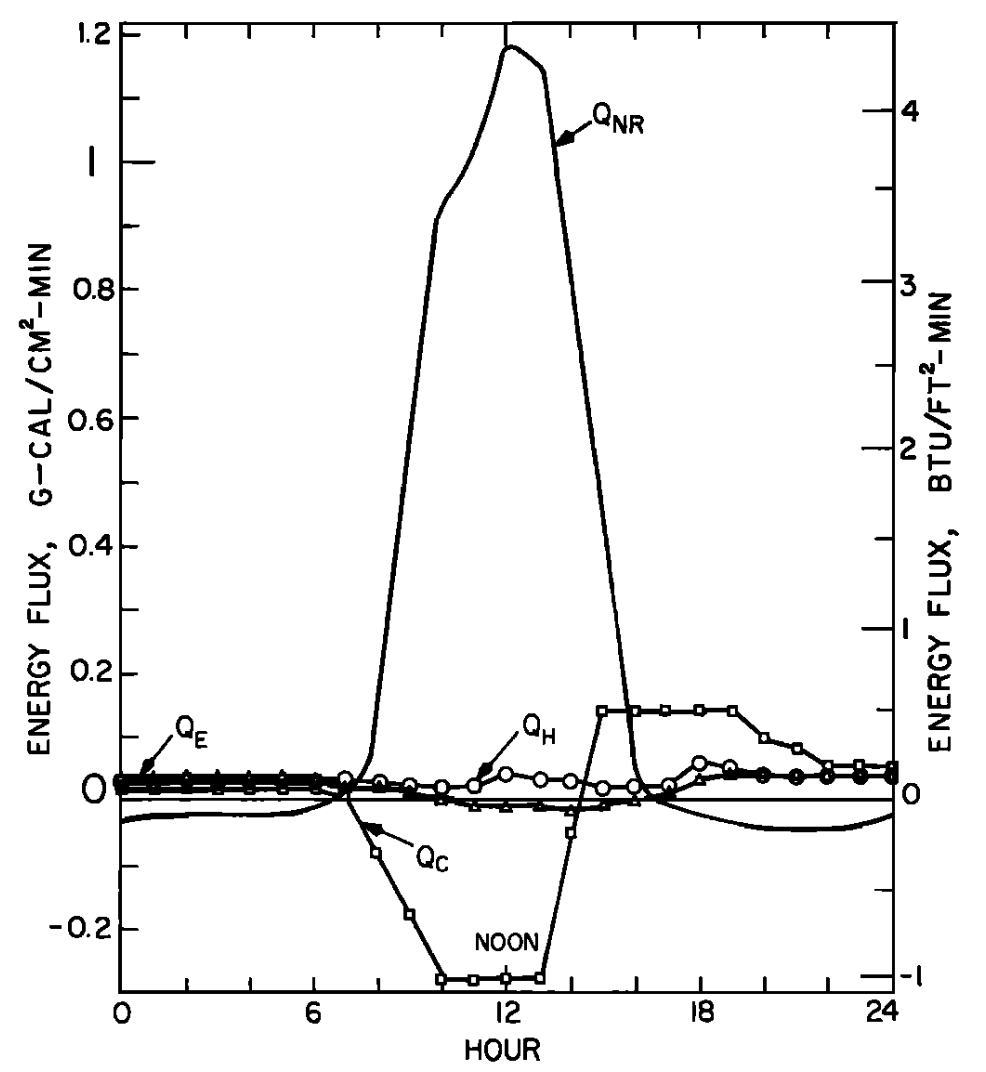
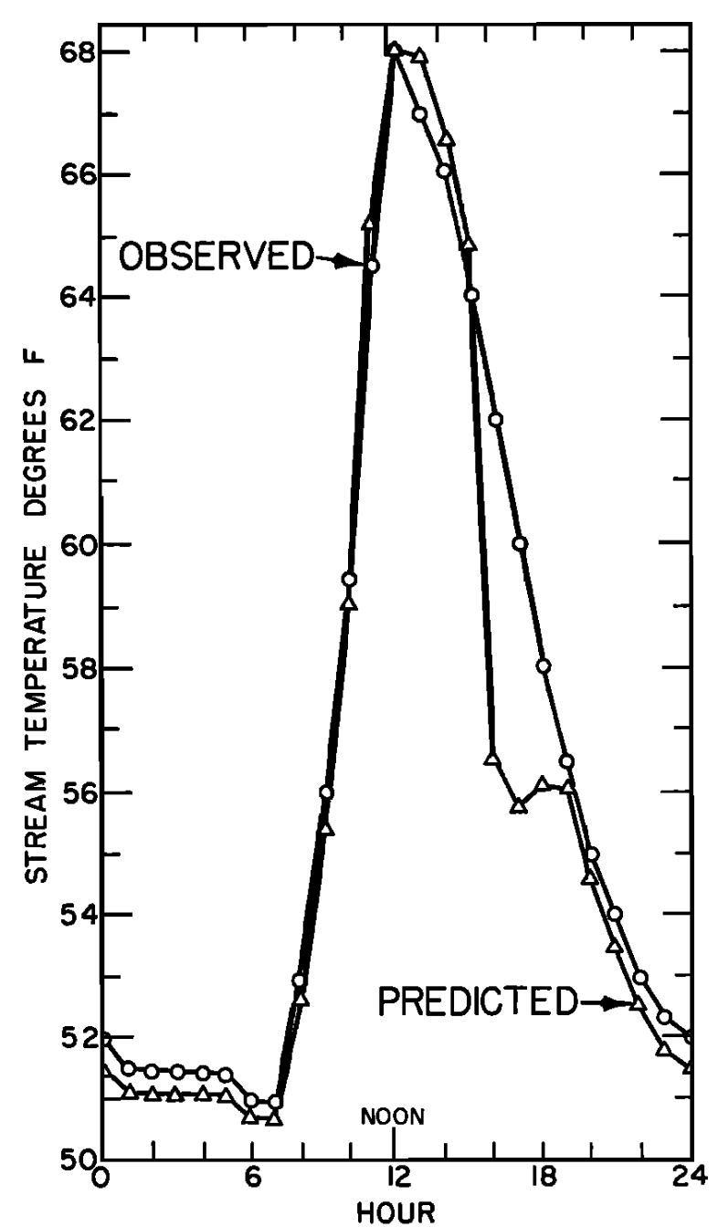
$a) The daily pattern in net thermal radiation ($Q_{NR}$), evaporation ($Q_E$), convection ($Q_H$), and conduction ($Q_C$) for the nonforested rock bottomed H. J. Andrews study section. From Brown, G. W. 1969. Pp. 73, 74. b) Observed and predicted hourly temperatures for the nonforested H.J. Andrews study section. From Brown, G. W. 1969, Pp. 73,74.$ $a) The daily pattern in net thermal radiation ($Q_{NR}$), evaporation ($Q_E$), convection ($Q_H$), and conduction ($Q_C$) for the nonforested rock bottomed H. J. Andrews study section. From Brown, G. W. 1969. Pp. 73, 74. b) Observed and predicted hourly temperatures for the nonforested H.J. Andrews study section. From Brown, G. W. 1969, Pp. 73,74.$

Figure 6.4: a) The daily pattern in net thermal radiation ($Q_{NR}$), evaporation ($Q_E$), convection ($Q_H$), and conduction ($Q_C$) for the nonforested rock bottomed H. J. Andrews study section. From Brown, G. W. 1969. Pp. 73, 74. b) Observed and predicted hourly temperatures for the nonforested H.J. Andrews study section. From Brown, G. W. 1969, Pp. 73,74.

To illustrate how the First Law can be applied to plant systems we will examine the heat balance of a leaf. The discussion is taken from Gates (1968). This is a natural first step towards understanding the heat balance of a plant because the leaf has a distinct geometry and, is the unit of photosynthesis. The First Law is used in a steady state condition ($\Delta U$ = 0) which assumes that the heat capacity of the leaf is not an important component of the heat fluxes. The heat balance is written \[\begin{equation} 0 = + Q_a - Q_e - C - LE \tag{6.15} \end{equation}\] where

$Q_a$ = radiant energy absorbed by the leaves ($W m^{-2}$),
$Q_e$ = radiation emitted by the leaves ($W m^{-2}$),
$C$ = convection flux ($W m^{-2}$),
and $LE$ = evaporative flux ($W m^{-2}$).

A positive sign indicates energy is being added to the system. Equation (6.15) describes completely the heat balance of a leaf. This is very important since the heat energy balance determines leaf temperature which affects the photosynthetic activity and shape of the leaf. A more complete analysis of the leaf system and the biological implications will be given in another module (Gates). In this module, it is most important to realize that we can write down the heat energy budget of the leaf and that there are four basic components to the heat balance: $Q_a$, $Q_e$, $C$, and $LE$.

To further illustrate the generality and wide application of the First Law, let us examine an animal as the system. Riechert and Tracy (1975) considered the thermal characteristic of the funnel web-building spider, Agelenopsis aperta. They hypothesized that reproductive success would be influenced by the microhabitat of the spider because this animal reproduces during the warmest season which is probably physiologically costly. More specifically, if A. aperta could spend more time on the web catching food, more young could be produced. The energy balance equation for the spider was assumed to be \[Q_a - Q_e - C = 0\] where

where $Q_a$ = radiant absorbed ($W m^{-2}$),
$Q_e$ = radiation emitted ($W m^{-2}$),
and $C$ = convection ($W m^{-2}$).

Of the three habitats considered the model predicts increasing thermal stress in the following order: mixed grassland depression, mixed grassland surface, and lava surface. Field observations have confirmed these predictions. Riechert and Tracy also found that the spiders did not randomly orient the direction toward which their funnels faced. In fact the general tendency was to face northerly which would eliminate direct solar radiation. Fig. 6.5 shows a plot of orientations and gives the mean direction. The tendency is strongest in Fig. 6.5c which shows all webs from unprotected sites.

To find out whether or not the energy budget influences the activity time of the spiders Riechert and Tracy measured spider activity. The barred region of Fig. 6.6 indicates when more than 50 percent of the spiders were active. This corresponds to a time of day when the body temperature of the spiders would be between 21 and 35 °C. This study emphasizes the importance of the thermal environment for A. aperta.

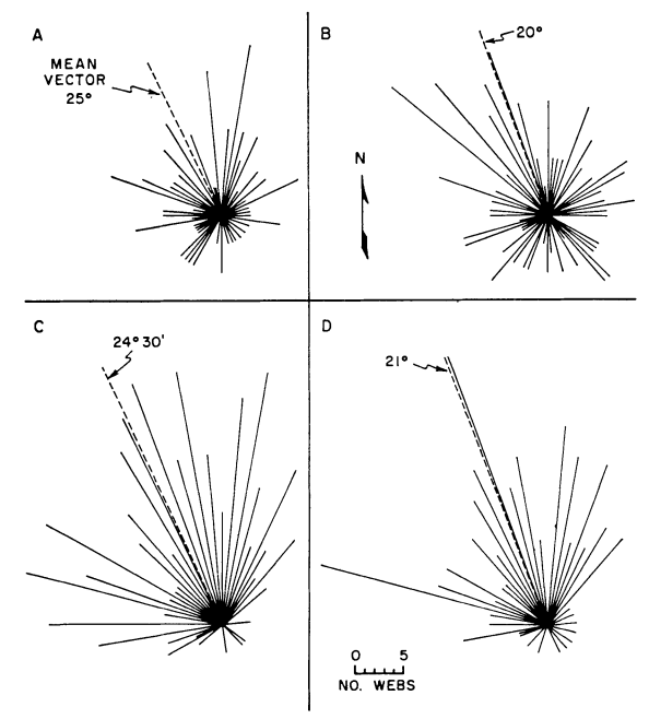
Funnel orientations for various habitats and sample groups in June 1971. (A) All webs in lava study area, (B) all webs in mixed-grassland study area, (C) all unprotected surface webs from all habitats, and (D) all webs from a rangeland plot lacking depressions and shrubs. Orientations represent compass directions to which the funnels face. From Riechert, S.E., and C. R. Tracy. 1975. P. 271.

Figure 6.5: Funnel orientations for various habitats and sample groups in June 1971. (A) All webs in lava study area, (B) all webs in mixed-grassland study area, (C) all unprotected surface webs from all habitats, and (D) all webs from a rangeland plot lacking depressions and shrubs. Orientations represent compass directions to which the funnels face. From Riechert, S.E., and C. R. Tracy. 1975. P. 271.

6.3.3 The First Law Generalized to Include Mass Flow

The final example we wish to consider is Lindeman’s (1942) work on the energy flow in Cedar Bog Lake. This is a classic paper describing the energy flow through an ecosystem. What we wish to point out is that a more general form of the First Law of Thermodynamics also encompasses the theory behind Lindeman’s research.

Lindeman (1941, 1942) provided information about the standing crop of eight categories: nanoplankton, net plankton, benthic plants, zooplankton, browsers, plankton predators, benthic predators, and swimming predators. He simplified his description of the aquatic ecosystem into three trophic levels as represented in Fig. 6.7. Losses were of two general types: mass losses from predation and respiration losses due to the energy required for maintenance of body tissues.

A more general version of the First Law is written in differential form as \[\begin{equation} d U = d \phi - dW \tag{6.16} \end{equation}\] where $d \phi$ includes both heat $dQ$ and mass changes $dM$. The change in any particular trophic level can then be viewed as a conservation of heat and mass energy. If we assume work changes are zero, the change in the internal energy of the $i^{th}$ trophic level (or organism is you wish) is equal to the sum of the j heat and/or mass fluxes \[\begin{equation} \sum_j d U_{ij} = \sum_j d M_{ij} + \sum_j d Q_{ij} \tag{6.17} \end{equation}\] If we consider the carnivores in Lindeman’s study as the $i^{th}$ trophic level, each prey item taken would be an increase in mass $M$. Heat exchange through the water is represented by a $Q$ term. Defecation products are usually the most important mass losses. Gallucci (1973) has reviewed the ecological literature and summarized this more general approach. Before passing on, it is important to realize that as equation (6.17) is written heat and mass fluxes are independent. Since many biology processes are temperature dependent, this is in general not true. Brett (1971) has provided an ecological example of the interaction of body temperature and food acquisition (also see problem 8). These kinds of interaction occur in plants also (Went 1957). Finally, since all life is far from equilibrium, in the sense of a thermodynamic system, classical representations do not always apply (e.g. Wilke 1975). Non-equilibrium theory, as discussed in later modules, is the first step toward handling these problems and it is an area of current research (Haken 1978, Lamprecht and Zotin 1978). A bibliography is included at the end of the module which, combined with the problems, should illustrate the pervasiveness of thermodynamics in biology.

Graph of percent of spiders active on the sheet with time of day on the mixed-grassland study area in midsummer (July and August) imposed on predicted spider temperature under these conditions and assuming a web-over-litter substrate. Barred area under flushability curve represents time periods during which over 50 percent of the individuals were active. Stippled area represents range of spider temperatures, exact temperature dependent upon amount of exposure to solar radiation. Upper boundary of predicted temperature curve signifies spider temperature if in full sunlight. Lower boundary signifies spider temperature if in full shade. Area enclosed by dashed lines represents body temperature range within which over 50 percent of the spiders are active. From Riechert, S. E., and C. R. Tracy. 1975. P. 272.

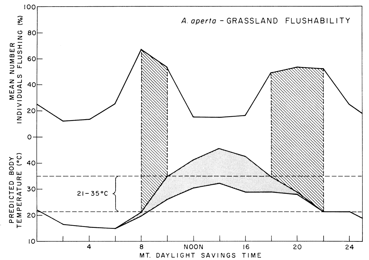
Figure 6.6: Graph of percent of spiders active on the sheet with time of day on the mixed-grassland study area in midsummer (July and August) imposed on predicted spider temperature under these conditions and assuming a web-over-litter substrate. Barred area under flushability curve represents time periods during which over 50 percent of the individuals were active. Stippled area represents range of spider temperatures, exact temperature dependent upon amount of exposure to solar radiation. Upper boundary of predicted temperature curve signifies spider temperature if in full sunlight. Lower boundary signifies spider temperature if in full shade. Area enclosed by dashed lines represents body temperature range within which over 50 percent of the spiders are active. From Riechert, S. E., and C. R. Tracy. 1975. P. 272.

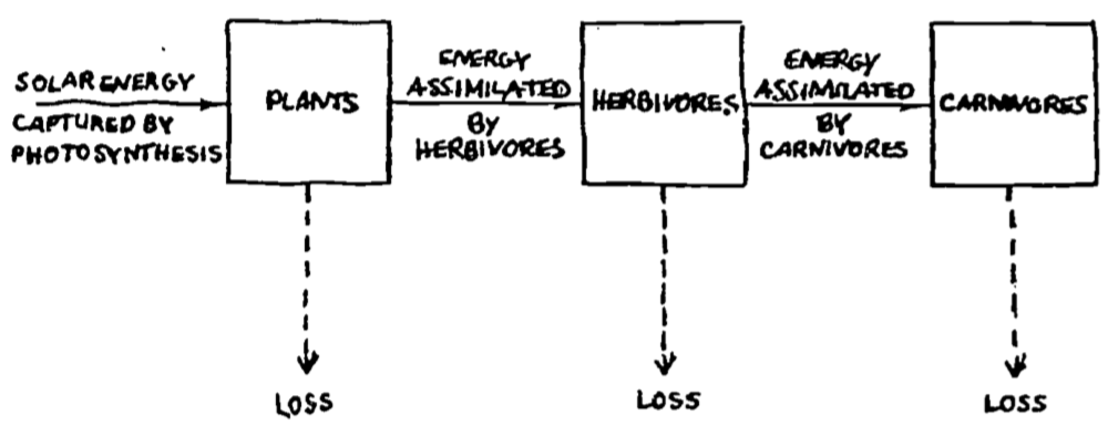
Figure 6.7: Lindeman’s (1941) analysis of energy flow in the Cedar Bog Lake ecosystem. From Williams, R. B. 1971. P. 546.

There are three important ideas in this module for the reader to remember: First, that the classical definitions and Laws of Thermodynamics can apply to all biological systems; secondly, that the First Law of Thermodynamics is a conservation of energy law that allows a researcher to describe mathematically the heat fluxes of any system of interest; finally, that the heat and mass energy balance of organisms have important ecological consequences that have been illustrated here and which offer challenging problems for scientists in the future.