1.4 The Definite Integral
The integration constant does not appear if the integral is a definite integral, written as
\[A = \int^b_a g(x)dx\] where \(a\), \(g\) are called the limits of the integral. In this case, the integral is determined by evaluating the antiderivative of \(g(x)\) at the values \(x = b\), \(x = a\) and subtracting. Thus, as with eqn. (1.3), if
\[\frac{df}{dx} = g(x)\]
then
\[\begin{align*} \int^b_a g(x)dx &= [f(x)]^b_a \\ &= f(b) - f(a) \end{align*}\]
Note that the integration constant is not written since it is eliminated through subtraction. If \(g(x) = 2x^2\), then \(\int g(x)dx = f(x) + C = 2x^3/3 + C\) and
\[\begin{align*} \int^b_ag(x)dx = \int^b_a 2x^2dx &= (2b^3 / 3 + C ) - (2a^3/3 + C) \\ &= 2b^3/3 - 2a^3/3 + C - C \\ &= f(b) - f(a) \\ \end{align*}\]
1.4.1 Area Under the Curve
Whereas the derivative can be used to represent the slope of a curve, the definite integral can represent the area under the curve (specifically, the area between the curve and the horizontal axis). For a curve given by \(y = g(x)\), the area (\(A\)) under the curve from \(x = a\) to \(x = b\) is written (see fig. 1.1).
\[ A = \int^b_a g(x) dx\]
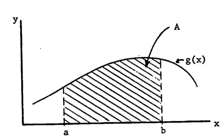
Figure 1.1: Area under the curve g(x).
This use of the definite integral has strong intuitive appeal. Consider the case where \(g(x) = 1\) as in figure 1.2.
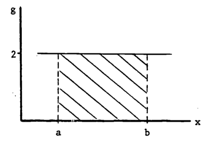
Figure 1.2: Area of Rectangle.
The area under \(g(x)\) is then
\[A = \int^b_a g(x)dx = \int^b_a 2 dx = 2 \int^b_a dx = 2(b-a)\]
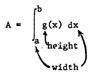
Thus \(\int^b_a dx\) represents the width and \(g(x)\) is the height. Thus the definite a integral as area has intuitive meaning: area = height \(\times\) width. In general, the same visual identification applies:
Example 1
Diffusion of a gas across a membrane is often described by Fick’s Law which states that the rate of transport is proportional to the product of the surface area of the membrane and the concentration gradient. Thus knowledge of the surface area is important. Certain leaves have nearly parabolic edges (fig. 1.3). The area of the top surface available for transport of water is then found by integrating the parabola function. If the dimensions of the leaf are length = 2a, width = 2b, then the parabola describing one edge is written
\[y(x) = -bx^2/a^2 + b\]
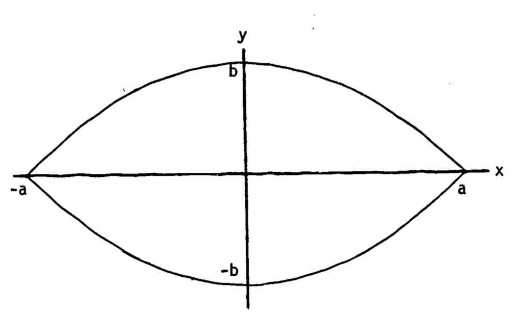
Figure 1.3: Leaf with parabolic edge contours.
The area of half the leaf is
\[ \frac{A}{2} = \int^a_{-a} (-bx^2/a^2 + b)dx \]
i.e., the area between the x-axis and the upper curve. Thus we calculate
\[\begin{align*} A &= 2 \int^a_{-a} (-bx^2/a^2 + b)dx \\ &= 2[-(b/a^2)x^3/3+bx]^a_{-a} \\ &= 2[(-ab/3 + ab ) - (ab/3 - ab)] \\ &= 8ab/3 \\ \end{align*}\]
We can use this equation to approximate the upper surface area of a Kalmia latifolia (mountain laurel) leaf. On average, the leaves are 8 cm long and 3 cm wide, thus a=4 and b=1.5, which we can use to solve for A.
\[\begin{align*} A &= 8ab/3 \\ A &= 8(4)(1.5) / 3 \\ A &= 16 cm^2 \\ \end{align*}\]
1.4.2 Improper Integrals
Occasionally we are interested in long term behavior of a measured quantity. For example, when raw sewage and other chemical pollutants are continually dumped into a lake, one effect is the rapid increase in the number of microorganisms. The resultant high level of organic oxidation from metabolism of the sewage can lead to extreme oxygen depletion of the lake, with obvious detrimental effects on other aquatic life (Dugan 1972). If we know something about the rate of oxygen consumption by the microorganisms, then we obtain the amount of oxygen consumed during a time period \(T\) by integrating the rate over that time period, i.e., using, a definite integral with limits 0, \(T\). We then estimate the maximum oxygen depletion by integrating over an infinite time interval. Such a definite integral with at least one infinite limit is called an improper integral.
Example 2
Assume that self-inhibition by the microorganism population causes the oxygen depletion to taper off as time becomes large. One model might be
\[\begin{equation} \frac{dC}{dt} = te^{-t^2} + e^{-t} \tag{1.4} \end{equation}\]
where \(C\) represents the quantity of oxygen consumed. A graph of \(dC/dt\) looks like figure 1.4.
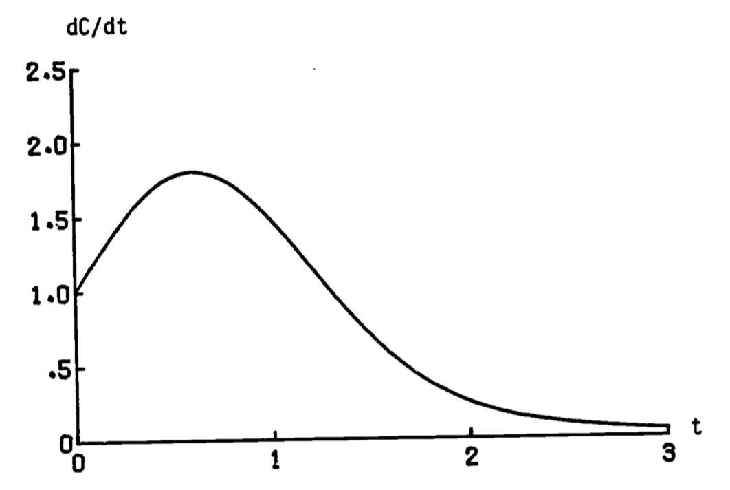
Figure 1.4: Rate of oxygen consumption.
The total amount of oxygen consumed by time \(T\) is then found by integrating eqn. (1.4).
\[C(T) = \int^T_0 (te^{-t^2} + e^{-t}) dt \]
The maximum depletion is then found by letting \(T\) increase to \(\infty\).
\[C(\infty) = \lim_{T \rightarrow \infty} \int^T_0 (te^{-t^2} + e^{-t}) dt \] With most nicely behaved models, we can evaluate \(C(\infty)\) directly. The above integral is then written
\[\begin{equation} C(\infty) = \int^\infty_0 (te^{-t^2} + e^{-t}) dt \tag{1.5} \end{equation}\]
and is evaluated as with previous definite integrals.
Some functions are not “nicely behaved” and certain integrals cannot be evaluated directly. If we desired to evaluate the circumference \(C\) of a tube with circular cross-section by using.an integral (instead of the well-known formula \(C = 2 \pi r\)) we can encounter difficulties. For one-quarter of the circle (fig. 1.5) the arc-length is given by (Schwartz 1974, p. 634)
\[ L = \int^r_0 \frac{r}{\sqrt{r^2-x^2}} dx\]
where \(r\) is the radius. The integrand is infinite at \(x=r\) (fig. 1.6). However, we can evaluate the integral by taking the limit of another integral:
\[\begin{align*} L &= \lim_{a \rightarrow r} \int^q_0 \frac{r}{\sqrt{r^2-x^2}} dx \\ &= \lim_{a \rightarrow r} [r \sin^{-1} (x/r) ]^a_0 \\ &= \lim_{a \rightarrow r} [r \sin^{-1} (a/r) ] = r\pi/2 \\ \end{align*}\]
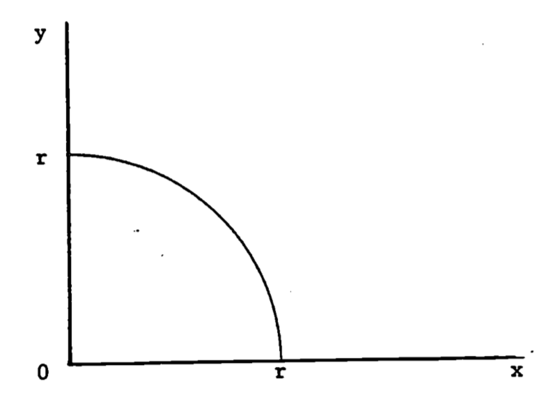
Figure 1.5: The quarter-circle, \(y=\sqrt{r^2 -x^2}\)
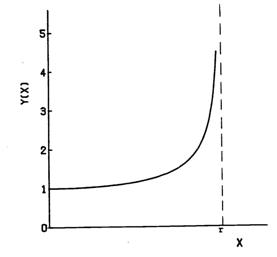
Figure 1.6: Integrand of arc-length formula, \(y=r/ \sqrt{(r^2 -x^2)}\)