2.4 Functions of Several Variable
2.4.1 Using Flow Diagrams
Flow diagrams can be used to help visualize the model being evaluated. The following example from A Biologist’s Guide to Mathematical Modeling in Ecology and Evolution by Otto and Day models the spread of a flu virus, using two populations: \(N(t)\) as the population with the flu, and \(S(t)\) as the population without (susceptible to) the flu.
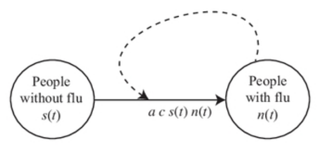
Figure 2.7: Flu Model
In the flu model, we assume that individuals with the flu interact with susceptible individuals at a rate proportional to \(N(t) S(t)\). Specifically, an infected individual has a probability \(c\) of contacting any \(S(t)\) susceptible individuals per day, giving a total number of contacts per day of \(c S(t)\) per infected individual. With \(N(t)\) infected individuals in the population, we expect a total of \(c N(t) S(t)\) contacts per day across the whole population. The probability that any one contact results in the transmission of the influenza virus is \(a\), and therefore we expect a total of \(a c N(t) S(t)\) new cases of flu per day.
To write a differential equation from this flow diagram, follow this “recipe”:
\[\frac{d(n(t))}{dt}=\mbox{the flow rates along arrows entering the circle + the flow rates along arrows leaving and returning to the circle - the flow rates along arrows exiting the circle}\] Using this recipe and the flow diagram, the resulting differential equations for the two populations are
\[\frac{d(N(t))}{dt}= a c N(t)S(t)\] \[\frac{d(S(t))}{dt}= -a c N(t)S(t)\]
2.4.2 Partial Derivatives
The oxygen model treated thus far involves one variable: oxygen uptake is given as a function of just the surrounding oxygen concentration. The population size depends only on time. A more complicated model, however, may involve many variables. Growth certainly depends on available food supply in addition to time. Oxygen consumption also depends on more factors than ambient oxygen concentration. One such model is discussed by Bayne, Thompson and Widdows (1973).
The model begins with the equation \[\begin{equation} \frac{dC}{dt}=aW^b \tag{2.3} \end{equation}\]
where \(C\) is the amount of oxygen consumed up to time \(t\), and \(a\), \(b\) and \(W\) are constants. The notation \(dC/dt\) demands that we may be able to consider \(C\) only as a function of \(t\). This is not always the case. Bayne, et al., studied mussels (Mytilus) with regard to the effects of food and temperature on oxygen consumption. One of their data sets gives values for the coefficients \(a\) and \(b\) for winter vs. summer at two activity levels:
Table 2.2. Oxygen consumption for Mytilus edulis
| Activity | |||
|---|---|---|---|
| Parameter | Season | standard | routine |
| a | Winter | 1.76 | 2.66 |
| Summer | 1.87 | 2.64 | |
| b | Winter | 0.724 | 0.774 |
| Summer | 0.67 | 0.702 |
Standard activity represents the resting state. Routine refers to the post-feeding time period where some filtration (i.e. muscle activity) is occurring. From table 2.2, we recognize significant dependence of “\(a\)” on the level of activity and dependence of “\(b\)” on both activity and season. Let season and activity be denoted \(s\) and \(m\), respectively. Then, in place of “\(a\)” and “\(b\)” we write \(a(m)\) and \(b(s,m)\) to show the dependence on the variables \(m\) and \(s\). Now \(C\), \(a\) and \(b\) are dependent variables and \(W\), \(s\), \(m\) and \(t\) are the independent variables. We must now write (2.3) as \[\begin{equation} \frac{\partial C}{\partial t}=a(m)W^{b(s,m)} \tag{2.4} \end{equation}\]
The derivative notation is different from that in (2.3) to indicate more than one independent variable. This derivative is called a partial derivative and represents the rate of change of \(C\) with time while all other variables are held constant. Note that by holding all of the independent variables (except \(t\)) constant, we also hold \(a\) and \(b\) constant. So this partial derivative is obtained by differentiating the function \(C\) with respect to \(t\) and treating all of the remaining independent variables as constants.
As a simple example, consider the function \[\begin{equation} y=xt^2 \tag{2.5} \end{equation}\] Then \[\frac{\partial y}{\partial x}=t^2\;\;\;\mbox{(t held constant)}\] and \[\frac{\partial y}{\partial t}=x\cdot 2t\;\;\;\mbox{(x held constant)}\]
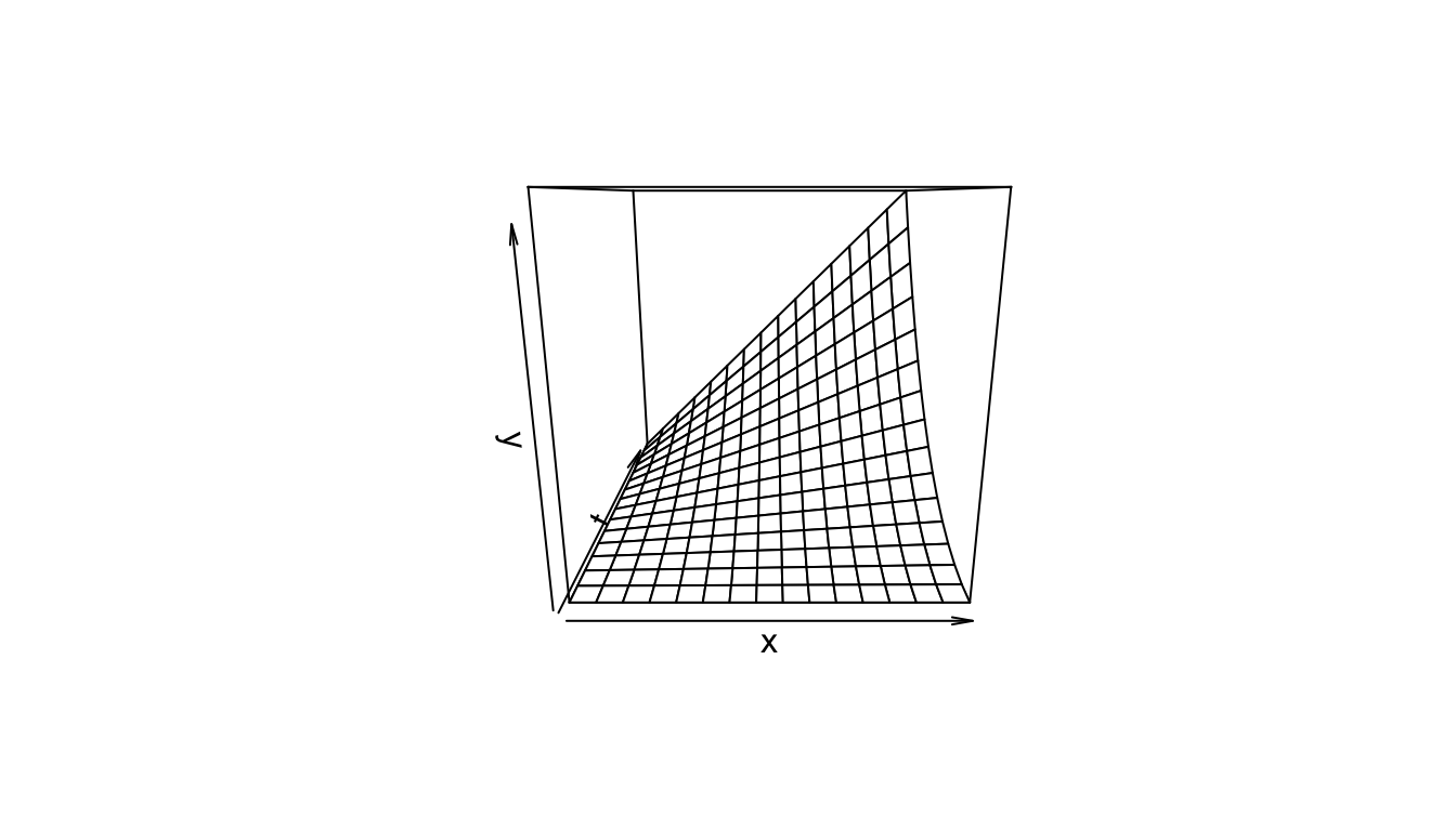
Figure 2.8: The function \(y=xt^2\).
A partial derivative is by nature merely one simple relation (of many) extracted from a complicated function. In (2.5), when both \(x\) and \(t\) vary, the graph of \(y\) vs. \(x\) vs. \(t\) is a three-dimensional surface (figure 2.8). When \(t\) is held constant, the graph (\(y\) vs. \(x\)) is a straight line (with slope \(t^2\) ); when \(x\) is held constant, the graph (\(y\) vs. \(t\)) is a parabola, as shown in Figures 2.9 and 2.10. These latter two graphs are much simpler than the surface of figure 2.8. Note that the straight line (\(y\) vs. \(x\)) is the far edge of figure 2.8a, and the parabola (\(y\) vs. \(t\)) is the near edge of figure 2.8c.
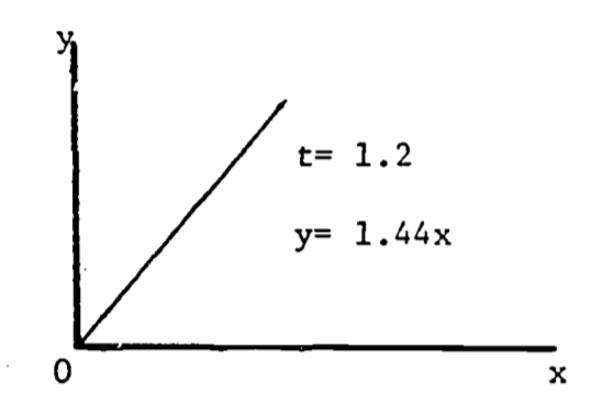
Figure 2.9: \(dy/dx=t^2\).
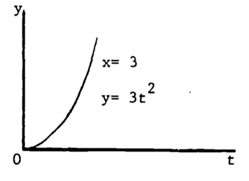
Figure 2.10: \(dy/dt=2xt\).
A more complicated example is the complete expression for equation (2.4) . The level of activity is based on the fraction of the maximal filtration rate. Then \(m=0\) represents the “standard” state, \(m=1\) gives the “active” state, and \(m=0.4\) is the “routine” state . Consider oxygen consumption during summer.
Then
\[a(m)=1.87(m+1)\]
and (2.3) becomes
\[\begin{equation}
\frac{\partial C}{\partial t}=1.87(m+1)W^{(0.7)}
\tag{2.6}
\end{equation}\]
Changes in “\(b\)” are not significant so that an average value, 0.7, can be used. Since (2.6) involves four variables, and thus cannot be plotted, we revert to the notation of (2.2), i.e., \(Q=\frac{\partial C}{\partial t}\). Then
\[\begin{equation}
Q=1.87(m+1)W^{(0.7)}
\tag{2.7}
\end{equation}\]
This last expression is similar in form to (2.5) and its graph has a similar shape. Problem 3 discusses (2.7) in more detail.
2.4.3 Critical Points in Three Dimensions
The extension of a critical point to functions of two variables is quite natural. A point \(P=(x_0,\;y_0,\;z_0)\) is a critical point for the function
\[z=f(x,y)\]
if
\[\frac{\partial f}{\partial x}=\frac{\partial f}{\partial y}=0\]
at the point \(P\). The classification of the critical point is, however, more complicated. Since there are three second derivatives, many cases could be considered:
\[\frac{\partial^2 f}{\partial x^2}=\frac{\partial(\partial f/\partial x)}{\partial x}\;\;\;\;\;\frac{\partial^2f}{\partial y^2}=\frac{\partial(\partial f/\partial y)}{\partial y}\]
\[\frac{\partial^2f}{\partial x\partial y}\equiv\frac{\partial(\partial f/\partial y)}{\partial x}=\frac{\partial(\partial f/\partial x)}{\partial y}\equiv\frac{\partial^2f}{\partial y\partial x}\]
This last “mixed” second derivative can be evaluated in either order only if the function \(f(x,y)\) is continuous in \(x\) and \(y\). The functions used in the examples which follow are continuous so that the order of differentiation is arbitrary. Rather than considering all combinations of sign (+, 0, -) in the second derivatives, we treat only three, which classify a relative maximum, relative minimum, and a saddle point. Define
\[L=f_{xx}(x_0,y_0)\cdot f_{yy}(x_0,y_0)-f_{xy}^2(x_0,y_0)\]
where
\[f_{xx}=\frac{\partial^2 f}{\partial x^2},\;\;\;\;\mbox{etc.}\]
P is a relative maximum if \(L > 0\) and \(f_{xx}(x_0,y_0)<0\).
P is a relative minimum if \(L > 0\) and \(f_{xx}(x_0,y_0)>0\).
P is a saddle point if \(L<0\).
When \(L = 0\), the situation is “undetermined” since its resolution is beyond the scope of this module.
An interesting example is the function \[z=x^3+y^3-3xy+15\] which seems to describe some of the properties of water falling across a rock face (Clow and Urquhart, 1974). Some of these properties are well known. The water will often dig potholes in the rock, especially if it falls onto a ledge. The corners and edges of the ledge eventually become rounded. We would then use a function which drops rapidly, levels off then drops steeply again. Figure 2.11 shows a three-dimensional computer plot of this function, looking across the origin into the positive octant (\(x>0\), \(y>0\), \(z>0\)). The required shape is evident, with the pothole just beginning to form. In fact, the function does possess a relative minimum at the point \((x, y, z) = (1, 1, 14)\). This model is discussed further in problem 6.
The saddle point in the waterfall model is located at the point \((0, 0, 15)\). The region around the saddle point represents the front part of the ledge. It is displayed in the computer-drawn graph of figure 2.12, expanded vertically to highlight the saddle shape. Some basic features of derivatives are shown here:
a) The slope changes from point to point.
b) The slope depends on the orientation of the tangent line. Thus, at a given point, the slope found by \(\partial z/\partial x\) may be different from the slope found using \(\partial z/\partial y\).
c) The slope at a relative maximum or relative minimum is zero, i.e. horizontal.

Figure 2.11: Waterfall function.
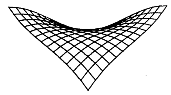
Figure 2.12: Saddle point of a waterfall function.