8.3 Black Body Radiation

In any discussion of radiative energy exchange, it is necessary to begin with an idealization of this process, which is described by the theory of black body radiation. This is rather awkward in the present instance since the biological implications of this abstraction from the real world are not immediately obvious. In fact, some of the most important aspects of biological systems result from their deviations from the idealizations of physics. For example, most organisms are not perfectly “black” in the physical sense of the word; that is, they do not absorb and emit radiation perfectly at all frequencies. The effect of the coloration of organisms will be to vary the degree to which the black body idealization can describe the system. However, it is the nature of science to explain in detail the simple system in the hope that the more complicated systems can be explained by small variations of the simple theory, and the expectation that the major results will be carried over to the more complicated systems. For radiative energy exchange this is precisely the case, and thus there is sufficient justification for presenting a discussion of black body radiation which, though not “simple” in the common sense of the word, is essential for an understanding of the more complicated systems which are the substance of biology.

The theory of black body radiation had a lengthy and fascinating development during the 1800’s, culminating in the work of Planck at the turn of the century. Many of the results discussed below were known at various stages during this period of repeated empirical research and hypothesis testing. However, the important results for biological applications can be derived directly from the formula of Planck, which mathematically (though not physically) culminated this field of experimental physics. The physical explanation of Planck’s formula awaited the work of Einstein, and ultimately the early founders of Quantum Mechanics.

Planck’s problem was to specify the energy distribution of the electromagnetic radiation within a cavity, the walls of which are atthermal equilibrium at the temperature $T$. That is, the problem is to find the energy density $E(\nu)$ ($J s m^{-3}$) of the radiation within the cavity between the frequencies $\nu$ and $\nu + d\nu$. The shape of the curve $E(\nu)$ vs. $\nu$ had been determined experimentally at various temperatures (Fig. 8.1). Planck found a solution to this problem in the form:

\[E(\nu)=\frac{8\pi h \nu^3 }{c^3}[e^{h\nu/ kT}-1]^{-1}\]

where $\nu$ is the frequency of the radiation, $T$ is the absolute temperature of the walls of the cavity, and $h$, $k$ and $c$ are physical constants (see symbols table). This energy distribution is called the black body energy distribution because it is the same as the energy distribution of radiation emitted by a perfectly black object which is at absolute temperature $T$. For measurement purposes, it is more useful to express this energy density in terms of the wavelength $\lambda$.

We can now plot out the energy density as a function of wavelength for different temperatures:

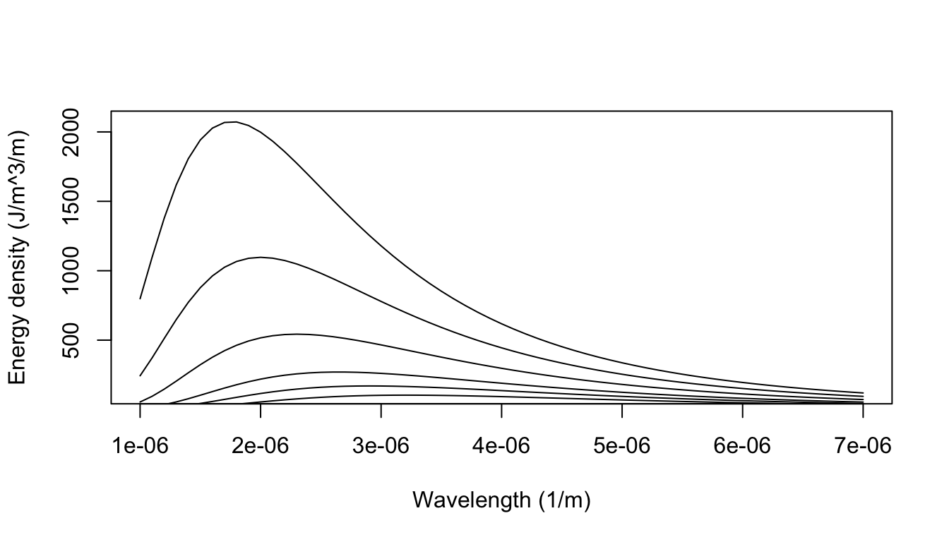
Figure 8.1: The blackbody radiation predicted from Plancks law closely aligned with that empirically observed (e.g., Lummer and Pringsheim 1901).

8.3.1 Wein’s Law of Shift

It can be shown that the $E(\lambda)$ distribution can be described by the wavelength $\lambda_m$ at which the distribution reaches its maximum. Qualitatively increasing the temperature $T$ shifts the maximum of the $E(\lambda)[E(\nu)]$ curve to a smaller $\lambda$ (higher $\nu$).

Example 1

The wavelength at which the energy density is a maximum at a given temperature $T$ can be found as follows:

\[E(\lambda)=\frac{8\pi hc}{\lambda^5}[e^{hc/\lambda kT}-1]^{-1}\] Make the substitution $u=hc/\lambda kT$: \[E(\lambda)=\frac{8\pi k^5T^5}{c^4h^4}[\frac{u^5}{e^u-1}]\] From calculus, the maximum can be found by solving:
$\frac{dE}{du}=0$, which gives \[\frac{dE}{du}=\frac{8\pi k^5T^5}{c^4h^4}[(5u^4)(e^u-1)^{-1}-e^u(u^5)(e^u-1)^{-2}]=0\] or \[[(5u^4(e^u-1)-u^5e^u)(e^u-1)]^{-2}=0\] which implies \[5u^4e^u-5u^4-u^5e^u=0\] or finally: \[e^{-u}+1/5u-1=0\] This transcendental equation can be solved by numerical techniques to give: \[u=4.9651....\] Thus \[\lambda_mT=\frac{hc}{uk}=2.8978\times10^{-3}mK=b\] b is called the Wien constant and the equation \[\lambda_m T=b\] is called Wien’s law of shift (1896 Wilhelm Wien). Therefore, the maximum of the black body curve $E(\lambda)$ at temperatures $T_1,T_2,T_3,...$ falls at $\lambda_1,\lambda_2,\lambda_3,...$ so that \[\lambda_1T_1=\lambda_2T_2=\lambda_3T_3=b\]

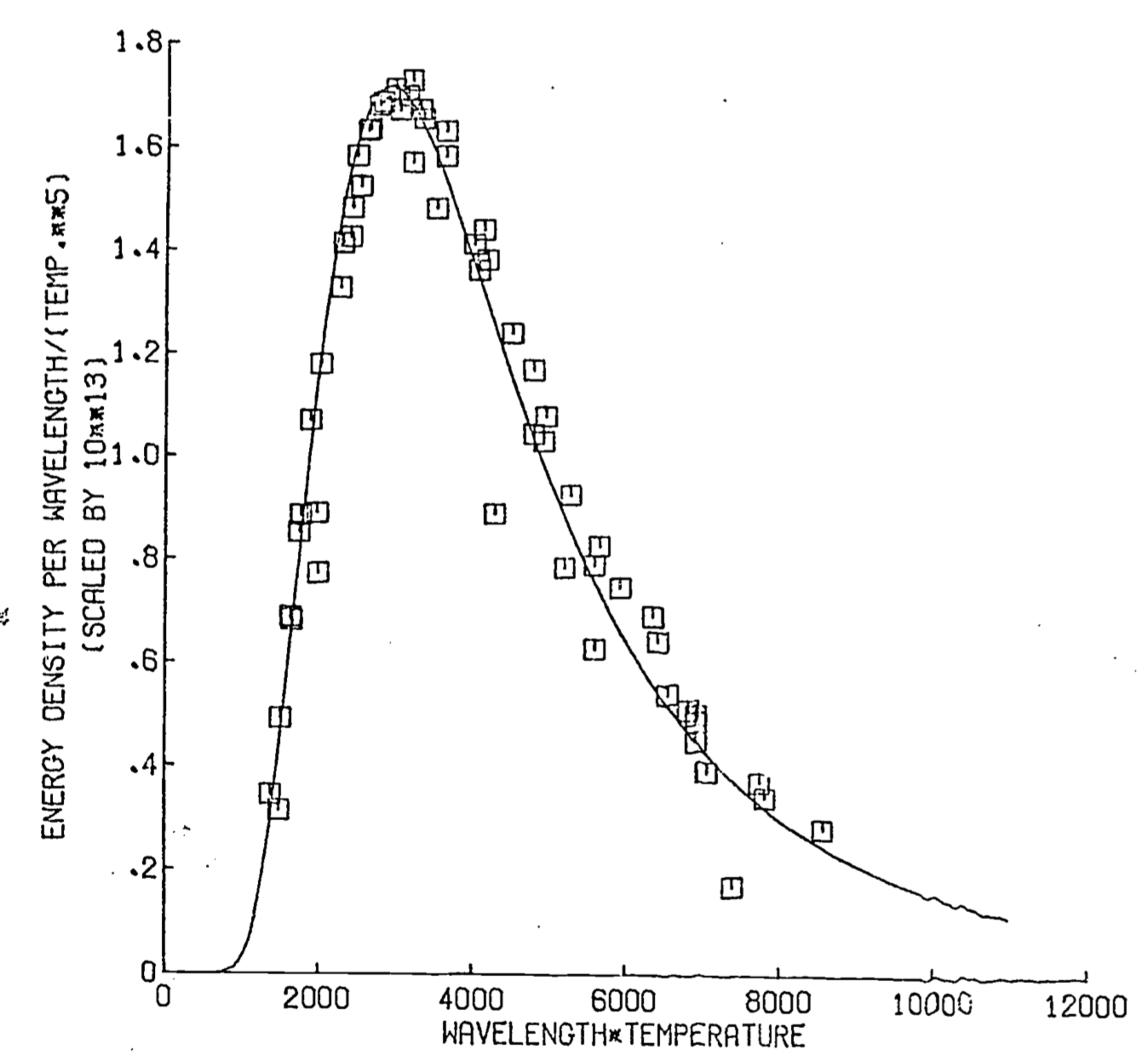
Figure 8.2: Wiens law- observed vs. predicted

The Wein law of shift is a very powerful result because it embodies a single relation between wavelength and absolute temperature. This is exemplified in the following problem.

8.3.2 Stefan-Boltzmann Law

If $E$ is the total energy density in all frequencies $(J m^{-3})$:

\[\begin{equation} E=\int_0^\infty E(\nu)d\nu=\frac{8\pi h}{c^3}\int_0^\infty\frac{\nu^3d\nu}{e^{h\nu/kT}-1} \tag{8.1} \end{equation}\]

Making a change of variable,
\[x=h\nu/kT \;\;\mbox{ which implies }\;\; dv=\frac{kT}{h}dx\]
Equation (8.1) becomes

\[\begin{equation} E=\frac{8\pi h}{c^3}(\frac{kT}{h})^4\int_0^\infty\frac{x^3dx}{e^x-1} \tag{8.2} \end{equation}\]

The value of the integral in Equation (8.2)

\[\begin{equation} I=\int_0^\infty\frac{x^3dx}{e^x-1} \tag{8.3} \end{equation}\]

can be obtained by numerical integration. This is a technique for approximating a definite integral by a finite sum. The value of the integral in Equation (8.3) can be found to be:

\[I=6.4983\]

Equation (8.2) can be re-expressed as \[\begin{equation} E=[\frac{8\pi h}{c^3}(\frac{k}{h})^4I]T^4=aT^4 \tag{8.4} \end{equation}\]

where the constant $a$ is equal to the value of the constants in the square brackets in Equation (8.4). The value of $a$ is found to be \[a=\frac{8\pi h}{c^3}\frac{k^4}{h^4}(6.4983)=7.5643\times10^{-10}Jm^{-3}K^{-4}\] The energy radiated by a black body per unit area per unit time, that is, the radiation emittance $E_n$, can be shown to be \[\begin{equation} E_n=\sigma T^4 \tag{8.5} \end{equation}\] where $E_n\equiv$ radiation emmitance and \[\sigma=(\frac{1}{4})ca=5.6693\times10^{-8}Wm^{-2}K^{-4}\] Equation (8.5) is called the Stefan-Boltzmann law and the constant $\sigma$ is called the Stefan-Boltzmann constant. Although Equation (8.5) is quantitatively precise, the functional relationship of the variables is more important than the exact numerical value of the constants. Of particular interest is that the radiation emittance is proportional to the fourth power of the absolute temperature.

The equation is of direct biological interest when it is realized that the Stefan-Boltzmann law governs the radiative energy exchange between an organism and its environment. Although this exchange of energy is usually not considered when calculating the energy budget of an organism, it can in some circumstances be a major factor affecting the heat balance of an organism. The following example and problem constitute a brief introduction to the application of this physical law to biology. For a more detailed exploration of this relationship, see modules 11 and 12.

Example 2

A bat with a surface temperature of 37°C is living in a cave which has walls at a temperature of 12°C. What is the radiation emittance of the bat? If the bat has a total surface area of 100 cm², what is its rate of heat loss by this process of radiative exchange?

Solution: Define

$T_0 \equiv$ the bat’s surface temperature (in K)
$T_a \equiv$ the ambient temperature (i.e., the temperature of the cave)(in K).

Clearly the bat is emitting radiant energy at the rate: \[E_0 = \sigma T_0^4\] and receiving radiant energy (from the walls) at the rate: \[E_a=\sigma T_a^4\] So the overall energy exchange by this process is given by: \[E=\sigma(T_0^4-T_a^4)\] with the convention that $E$ is positive when the overall radiation balance is such that the bat is emitting more than it absorbs; i.e., it is losing energy to the environment at the rate $E$.

For this example: \[T_0 = (273+37)K = 310K\] \[T_a=(273+12)K=285K\] which gives an energy emmitance of: \[\begin{align*} E&=5.67\times10^{-8}(Wm^{-2}K^{-4})[(300k)^4-(285K)^4] \\ &=5.67\times10^{-8}[9.235\times10^9-6.598\times10^9]Wm^{-2} \\ &=5.67[92.35-65.98]Wm^{-2} \\ &=149.5Wm^{-2} \\ \end{align*}\] The bat’s total heat loss rate $H$, by this process is \[H=E(SA)\] where $SA$ = surface area, so \[\begin{align*} H&=149.5Wm^{-2}(100cm^2) \\ &=1.495W \\ \end{align*}\] Although in this example the heat loss rate was relatively small, when there are larger differences between the organism’s temperature and the (radiation) temperature of the environment, the heat loss rate can be quite high. This situation pertains in the following problem.

8.3.3 The solar constant

A physical parameter which imposes a significant constraint upon the evolution of terrestrial organisms is the amount of energy generated by the sun which is intercepted at the earth’s surface. Almost all of the energy which drives the biological processes on the earth comes directly or indirectly from the sun. Thus the amount of the sun’s energy that the earth receives is of interest for at least two reasons: (1) This is the upper limit to the amount of energy that could be absorbed by a surface and turned into heat. (2) This is the upper limit to the amount of energy that could be converted by a photosynthetic unit into chemical energy. Since the actual amount of sunlight available at the earth’s surface is dependent upon absorption by the atmosphere, and thus on such variables as latitude, the sun’s altitude in the sky (see module 11, section on Direct Solar Radiation), or cloudiness, the measure of the sun’s energy available at the earth is determined instead for a unit area just outside the earth’s atmosphere. This measure of the sun’s energy (actually the rate of the available energy, i.e., power) is called the solar constant.

The solar constant can be calculated theoretically from the Stefan-Boltzmann law and conservation of energy. Assuming the sun to be a black body with a surface temperature $T_s$, by the Stefan-Boltzmann law, its radiation emittance (energy radiated per unit area per unit time) is given by:

\[\begin{equation} E_s=\sigma T_s^4 \tag{8.6} \end{equation}\]

Thus the total power emitted by the sun can be found by integrating $E_s$ over the sun’s surface. Since $T_s$ is (assumed to be) constant, this is equivalent to multiplying the constant $E_s$ by the surface area of a sphere with the sun’s radius ($r_s$). The total power is given by:

\[\begin{equation} E=4\pi r_s^2 E_s \tag{8.7} \end{equation}\]

By conservation of energy, if no energy is lost in the intervening space, all of the radiation emitted radially out from the sun will be intercepted by an (imaginary) sphere centered on the sun with a radius equal to the mean distance from the sun to the earth ($r_E$). The power flow per unit area ($E_E$) across this (imaginary) sphere will be equal to the total power available ($E$), divided by the surface area of the sphere ($4\pi r_E^2$). That is,

\[\begin{equation} E_E=E/4\pi r_E^2 \tag{8.8} \end{equation}\]

Substituting Equation (8.7) in Equation (8.8) gives

\[\begin{equation} E_E=\frac{4 \pi r_s^2E_s}{4\pi r_E^2}=\frac{r_s^2}{r_E^2}E_s \tag{8.9} \end{equation}\]

The quantity $E_E$ which is the power available (per unit area per unit time) on a surface at the earth’s distance from the sun, is the parameter of interest, the solar constant. Inserting Equation (8.6) into Equation (8.9) gives immediately:

\[\begin{equation} E_E=(\frac{r_s^2}{r_E^2})\sigma T_s^4 \tag{8.10} \end{equation}\]

We can use the above equation equationand the following physical parameters to calculate the solar constant: \[\begin{align*} T_s&=5700K \\ r_s&=7.1\times10^8m \\ r_E&=1.49\times10^{11}m \\ \sigma&=5.6693\times10^{-8}Wm^{-2}K^{-4} \\ \end{align*}\]

$E_E=1.3610^3 Wm^{-2}s{-1}

When we convert to $cal\cdot cm^{-2}min^{-1}$, our solar constant is $1.95 cal\cdot cm^{-2}min^{-1}$.