1.7 Differential Equations

As was previously mentioned, the integral is also used to solve a differential equation. In the simplest form, if an equation is written as $$\frac{dx}{dt} = f(t)$$ then the solution (general solution) is $$x(t) = \int f(t)dt$$ If we know the value of $x$ at $t = 0$, the initial condition, then the differential equation has a unique solution given by $$x(t) = \int^t_0 f(\tau)d \tau + x(0)$$

1.7.1 Separation of Variables

When the differential equation also involves $x$ on the right-hand side, the solution is not so easily represented. Other techniques must then be employed to represent the problem by a set of integrals whose integrands are functions of only the variable of integration. One such technique is separation of variables.

Example 9

Let us return to example 4. The equation is

$$\begin{equation} \frac{dN}{dt} = rN(1 - N/K) \tag{1.19} \end{equation}$$

The simple representation given above fails here: $$N(t) = \int rN(1 - N/K)dt$$ To integrate, we need to know $N$ as an explicit function of $t$, which of course we do not know. However, by multiplying both sides of eqn. (1.19) by the differential $dt$, we obtain $$dN = rN(1 - N/K)dt$$

and by dividing by $N(1 - N/K)$ we successfully separate the variables $N$, $t$ on either side of the equality: $$\frac{dN}{N(1- N/K)} = rdt$$

Integration is now possible since each integrand is a function of just the variable of integration. $$\int \frac{1}{N(1- N/K)} dN = \int rdt$$

How are initial conditions incorporated now? Since the indefinite integral produces an integration constant, the constant is determined by the initial condition, making the general solution unique.

Example 10

A recent study on water purification (Dickson, et al, 1977) included the mortality of fish due to intermittent chlorination. The following data were obtained (Table A) where frequency is the number of doses per 24 hours.

Table A. Fish Mortality Due to Intermittent Chlorination

Mortality	Frequency	Duration (hr)
0.01	1	1.5
	2	0.7
	4	0.3
0.10	1	3.2
	2	1.4
	4	0.7
0.20	1	4.3
	2	2.0
	4	0.9
0.50	1	7.5
	2	3.4
	4	1.6

A mathematical model has been devised which shows the effect of duration ($T$) and frequency ($F$) on mortality ($M$) using two differential equations:

$$\begin{equation} \partial M / \partial T = a_1T^{1.5} \tag{1.20} \end{equation}$$

$$\begin{equation} \partial M / \partial F = a_2 F^{1.8} \tag{1.21} \end{equation}$$

where $a_1$ is a function of $F$ and $a_2$ is a function of $T$. Another model was derived by curve fitting, using Table A and is quite different. For a given $M$,

$$\begin{equation} \ln(T)=b_1 - b_2 \ln F \tag{1.22} \end{equation}$$

where it is now assumed that $b_1$ is a function of $M$: $$b_1 = 2.16 + 0.40 \ln M$$

Can both of these models hold? Are they consistent? We can answer this by integrating the first model to derive a single expression for $M$ as a function of $F, T$. Each equation (1.20), (1.21) involves a single partial derivative, so that one of the variables can be assumed constant. By holding $F$ constant, we integrate eqn. (1.20) to obtain $$M = (a_1/1.5)T^{2.5} + C_1$$ which is more precisely written, with $a_1$ as a function of $F$, as

$$\begin{equation} M = \frac{a_1(F)}{1.5}T^{2.5}+C_1 \tag{1.23} \end{equation}$$

Similarly, we integrate eqn. (1.21) with respect to $F$, holding $T$ constant.

$$\begin{align*} M &= \int a_2 F^{1.8} dF = (a_2 / 1.8) F^{2.8} + C_2 \\ &= \frac{a_2(T)}{1.8} F^{2.8} +C_2 \\ \end{align*}$$

Thus $$\frac{a_1(F)}{1.5} T^{2.5} +C_1 = \frac{a_2(T)}{1.8}F^{2.8} +C_2$$

We assume no observable mortality if no chlorination occurs, so that, if $F = 0$ or $T = 0$, then $M = 0$. Thus $C_1= C_2 =0$. $$\frac{a_1(F)}{1.5} T^{2.5} = \frac{a_2(T)}{1.8} F^{2.8}$$ Therefore, we must conclude that $$a_1(F) = 1.5C F^{2.8}$$ $$a_2(T) = 1.8C T^{2.5}$$ where $C$ is some proportionality constant. From eqn. (1.23) we have

$$\begin{equation} M = C F^{2.8} T^{2.5} \tag{1.24} \end{equation}$$

It is now straightforward to manipulate eqn. (1.22) to look like eqn: (1.24). $$\ln T = (2.16 + 0.40 \ln M) - b_2 \ln F$$ $$\frac{\ln T + b_2 \ln F - 2.16}{0.40} = \ln M$$ $$\frac{\ln T + ln(F^{b_2}) - \ln(e^{2.16})}{0.40} = \ln M$$ $$2.5 \ln (TF^{b_2}/8.7) = lnM$$ $$\ln[(TF^{b_2} /8.7)^{2.5} ] = \ln M$$ $$T^{2.5} F^{2.5b_2} /(8.7^{2.5} ) = M$$ Thus, $b_2 = 2.8/2.5 = 1.1, \;\;C = 1/(8.7)^{2.5} = 0.0045$ and the models agree.

1.7.2 Residual Norm

Often a differential equation cannot be solved by any standard methods and an approximate solution is developed. In some cases, bounds on the error in the approximation can be derived. Too often, however, calculating the error bounds is as complicated as determining the solution itself. A recent idea is to use the least-squares norm (or occasionally some other norm) as a gauge of the accuracy of the approximation. With only the differential equation at hand, a new type of norm, the residual norm, is used.

Consider a differential equation written as $$\frac{dx}{dt} = f(x,t)$$

with initial condition $x(0) = x_0$. If the equation is rewritten as $$dx/dt - f(x,t) = 0$$

then we obtain an expression which vanishes when the exact solution is used. In operator notation the equation is $$L(x,t) = 0$$ where $L$ is the differential operator defined by $$L(x,t) = dx/dt - f(x,t)$$ If $L$ operates on an approximate solution, $\overset\sim x (t)$, then $L(\overset\sim x) \neq 0$, and its value is the residual. Yet we would expect $L(\overset\sim x)$ to be small if $x$ is a good approximation. The final step is to decide on some interval over which the approximation’s accuracy is to be judged, say $[a,b]$. Then the least-squares residual norm for the approximate solution $\overset\sim x (t)$ is $$\| R(\overset\sim x) \|_2 = [\int^b_a (L(\overset\sim x,t))^2 dt]^{1/2}$$

Note that $\| R(\overset\sim x) \|_2 = 0$ if the exact solution is used, since $L$ is then 0. This limiting behavior suggests the residual norm as a qualitative indicator of the accuracy of an approximate solution. No theory exists, however, for estimating the actual error from the value of the residual norm.

Example 11

A deer population is threatened by severe storms as well as reduced grazing area due to a small fire. Consequently, a moratorium on deer hunting is imposed until the deer population returns to 60% of the carrying capacity for the area. How long should the moratorium be imposed?

Assumptions are now presented which allow us to model the population dynamics of the deer and estimate the duration of the moratorium. Let the logistic growth model be used: $$\frac{dn}{dt} = Rn(1-n/K)$$

Assume that the current population size is 400, the carrying capacity ($K$) is 2000, the intrinsic growth rate ($R$) is 1.0 and that the approximate solutions should be fairly accurate for the first three years. Assume also that the moratorium is not obeyed immediately, so that hunting pressure gradually tapers off. Let the growth model with the “harvesting” (i.e. hunting) term be

$$\begin{equation} \frac{dn}{dt} = Rn(1-n/K) - e^{-t}n \tag{1.25} \end{equation}$$

with initial condition $n(0)-n_0$.

Assume also that you do not have access to either a programmable calculator or a computer. This equation cannot be solved by separation of variables (try it), so some approximation must be made. From previous studies, you learn that the following two models have been used fairly successfully to model short term population growth.

$$\begin{equation} n_1(t) = (K-n_0)(1-e^{-Rt/5} ) + n_0 \tag{1.26} \end{equation}$$

$$\begin{equation} n_2(t) = n_0 e^{Rt/3} \tag{1.27} \end{equation}$$

Note that $n_1(t)$ tapers off at the carrying capacity, but $n_2(t)$ is exponential growth for $n_2 \approx 0$; both are properties the exact solution must possess. Which approximation is better? We compare $n_1$ and $n_2$ by evaluating their least-squares residual norms. Rewrite eqn.(1.25) as $L(n) = 0$, where $L(n)$ represents the differential operator acting on $n$: $$L(n) = dn/dt - Rn(1-n/K) + e^{-t}n = 0$$

We expect a good approximate solution, $n_a$, to give $$L(n_a) \approx 0$$ and thus its residual norm should also be small: $$\| R(n_a) \|_2 \equiv [\int^T_0 (L(n_a))^2 dt]^{1/2} \approx 0$$ Intuitively, the smaller $\| R \|_2$ is, the better the approximation should be. For this example, assume the following values: $$K = 2000, \; R=1, \; n_0=400, \; T=3$$

The integrands in $\| R(n_1) \|_2$ and $\| R(n_2) \|_2$ are now calculated. From eqn. (1.26) we obtain, after a few steps,

$$\begin{equation} [L(n_1)]^2 = (2000 e^{-t}- 1600 e^{-1.2t} + 1280 e^{-0.4t} -2800 e^{-0.2t} +1600)^2 \tag{1.28} \end{equation}$$

From eqn. (1.27) we obtain

$$\begin{equation} [L(n_2)]^2=[ (400/3) e^{t/3} - (1-400 e^{t/3}/2000 -e^{-t}) 400 e^{t/3}]2 \tag{1.29} \end{equation}$$

After multiplying out the square in each equation and collecting terms, we can write both (1.28) and (1.29) as sums of exponential functions, and thus both can be integrated by hand easily (but tediously). The results are, upon integrating over the interval $[0,3]$: $$\| R(n_1) \|_2 = 661.8$$ $$\| R(n_2) \|_2 = 172.3$$ Figure 1.19 shows the accuracy of the two approximate solutions as compared to a numerical solution to the original differential equation (1.25). It appears that, for the chosen values of $R$, $K$ and $n_0$, the approximation $n_2(t)$ is better, and the residual norm for $n_2$ supports this evaluation. The 60% of carrying capacity, i.e. 1200, is reached in 3.30 years using $n_2(t)$, and in 3.08 years according to the numerical solution $n(t)$. It is interesting that, without the term for hunting (curve $n_0(t)$ in fig. 1.19), the population reaches the 60% level in only 1.79 years.

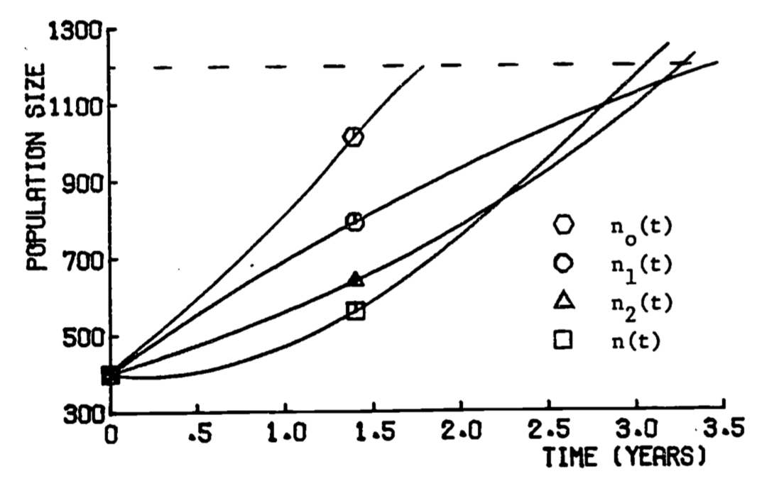
Figure 1.19: Approximate growth functions

---