10.4 The Operative Environmental Temperature

Models of the physical processes that govern the heat energy exchange of animals involve many environmental as well as organismal parameters which make the results difficult to summarize. One must use the four heat transfer processes (radiation, convection, evaporation and conduction) to link the microclimate (air temperature, wind speed, etc.) to the animal’s physiology, behavior and morphology. With such a large number of independent variables, it is apparent that it would be helpful to have a single number that would allow one to say how the animal “felt” in that environment. At first this may seem difficult. For example, if all the environmental variables and homeotherm’s thermoregulatory actions are fixed, the organism will have a specific metabolic rate. It is possible, however, to change the external conditions–say reduce the body-air temperature difference but increase the wind speed so that the organism will have the same metabolic rate to maintain thermal equilibrium or one could lower the air temperature but increase the absorbed radiation so that a poikilotherm would not have a different body temperature. The concept of operative environmental temperature lets one say quantitatively which environments are equivalent thermodynamically for the organism. Because this concept undercuts the physical processes, valuable information is lost about the animal’s coupling to the environment. But indeed this is the purpose of the operative environmental temperature. It may actually be that animals respond to a stimulus that has already integrated all the thermal fluxes.

10.4.1 Mathematical Development of the Operative Environmental Temperature

In this section, I develop the operative environmental temperature ($T_e$) as Bakken and Gates (1975) presented it. A discussion and summary of alternative formulations can be found in Bakken (1979a) about which I will comment briefly later.

I will begin with a simple model that approximates a homeotherm. The heat transfer processes and heat sources included are absorbed radiation, reradiation, convection, respiratory and cutaneous water loss and metabolism. Applying the First Law of Thermodynamics to the surface of the animal at temperature $T_r$ shows that \[ \mbox{Energy In} = \mbox{Energy Out}\] and thus \[\begin{equation} Q_{a} + K ( T_b - T_r ) = Q_{e} + C + E_r. \tag{10.2} \end{equation}\] The first energy in term $Q_a$ is absorbed thermal and solar radiation. The second term is conductance through the animal as a function of the gradient between internal body temperature $T_b$ and surface temperature $T_r$, where $K$ is thermal conductance of the organism. The energy out terms correspond to emitted thermal radiation $Q_{e}$, convective heat exchange with the air $C$, and evaporative heat loss from the outer surface $E_r$.

The heat balance at the core of the animal can be likewise expressed as \[\begin{equation} M-E_b= K ( T_b - T_r ), \tag{10.3} \end{equation}\] where $M$ is metabolism and $E_b$ is the evaporative heat loss from the respiratory system.

We then further consider the energy balance at the animal’s surface. The rate at which heat is emitted from the organism’s surface is given by the Stefan-Boltzman Law: \[Q_e= \sigma \epsilon T_r^4,\] where $\sigma$ is the Stefan-Boltzmann constant ($5.67 \times 10^{-8} W m^{-2}K^{-4}$) and $\epsilon$ is the thermal emissivity of the organism’s surface.

We can use a Taylor-Series approximation to linearize the heat transfer, expanding about the mean surface temperature $T_r$ as \[{T_r}^4 \cong {\overline{T}_r}^4 + 4{\overline{T}_r}^3 (T_r - \overline{T}_r) = (4{\overline{T}_r}^3) T_r - 3{\overline{T}_r}^4\] We can thus approximate $Q_e$ as \[\sigma \varepsilon {T_r}^4 \cong (4 \sigma \varepsilon {\overline T_r}^3)T_r - 3 \sigma \varepsilon {\overline T_r}^4.\] For convenience, we follow Bakken and Gates (1975) and let $4 \sigma \varepsilon {\overline T_r}^3 = R$ and define $Q_n$ as the net rate of heat tranfer by all radiative processes. Thus, $Q_n = Q_a + 3 \sigma \varepsilon {T_r}^4$. Equation (10.2) can then be rewritten as \[\begin{equation} Q_n + K(T_b - T_r) = R T_r + h_c (T_r - T_a) + E_r \tag{10.4} \end{equation}\] Equations (10.3) and (10.4) are then solved simultaneously to eliminate the surface temperature $T_r$. The rationale for this manipulation is the one not really concerned with the surface temperature. The question is: How are the animal’s body temperature and physiological processes being influenced by the thermal environment? Completing the elimination yields \[\begin{equation} T_b = \frac{h_c T_a + Q_n}{R + h_c} + (M - E_b) \frac{K + h_c + R}{K(h_c + R)} - \frac{E_r}{R+ h_c} \tag{10.5} \end{equation}\]

The important point of equation (10.5) is that the first term of the right-hand side does not depend on any physiological processes. It measures the component of the body temperature that is strictly due to the physical environment. This is the term Bakken and Gates (1975) labeled the operative environmental temperature, $T_e$. They say

Te may be identified as the temperature of an inanimate object of zero heat capacity with the same size, shape and radiative properties as the animal and exposed to the same microclimate. It is also equivalent to the temperature of a blackbody cavity producing the same thermal load on the animal as the actual non-blackbody microclimate, and therefore may be regarded as the true environmental temperature seen by that animal.

Bakken (1976a,b) and Bakken and Gates (1975) have extended these ideas in several ways. Most importantly they show that more complicated models including conduction can be incorporated into this same framework. Second, as Bakken (1976a) notes, the operative environmental temperature strictly speaking is not a temperature. This is because two systems are said to have the same temperature if each is in thermal equilibrium with a third system (Stevenson 1977a, Zemansky and Van Ness 1966). If the animals were of different size, the convection coefficient would be different and the two $T_e$s would not be equal. Yet each model organism would be in thermal equilibrium with the microclimate but not each other. Therefore, the zeroth law is not satisfied. This, however, is not a drawback for the use of $T_e$ in temperature regulation studies.

Bakken (1976a), following Gagge (1940), has made the further complication of introducing the standard operative environment temperature. He felt this step was necessary so that the primary physiological response of animals to their thermal environment (metabolic rate minus evaporative water loss) could be unambiguously defined in a metabolic chamber. Although it was the purported intention of the operative environmental temperature to incorporate all the effects of the thermal environment into one stress index, the standard operative environmental temperature was created because the overall heat transfer coefficient between the animal and the environment (see $K_0$) must uniquely define for the effective dry heat production to be predicted. The overall conductance depends on wind speed and the thermal properties of the underlying substrate which can be standardized in metabolic chambers. The approach has the advantage of being able to relate laboratory experiments to field studies as well as decreasing the differences environmental temperature are found in Bakken (1976a, pp. 357-367).

Unfortunately, like the operative environmental temperature, this concept has limitations which Bakken (1976a) discusses. In particular, it is assumed that body temperature, posture, orientation and blood flow rates are constant. This is not necessarily the case. Simply the stress state of the animal may increase metabolic rates. Furthermore, this formulation does not account for the differences in water loss rates due to effects of changing ambient water vapor concentration (see Bakken 1979a for references including this effect).

One final comment is necessary before proceeding. Bakken and Gates (1975) approximated the heat transfer between the animal and environment by linearizing about the mean surface temperature. Robinson et al. (1976) gave two derivations linearizing about air temperature and about the operative environmental temperature. Bakken (1979a) has evaluated the errors in these different approaches and finds that only in the case of naked animals do any of the alternatives give poor results. He further presents a procedure using numerical techniques to get exact results which is important for calculations of the heat balance of naked animals or in simulation studies where errors can accumulate.

TrenchR offers several strategies for estimating operative environmental temperatures of organisms that have reached an equilibrium with their environment (“steady-state”, no heat retention). The following function uses the equations in the chapter on heat transfer (module 7) above to solve the energy balance for $Te$ (K).

library(TrenchR)

Tb_Gates(A=1, D=0.001, psa_dir=0.6, psa_ref=0.4, psa_air=0.6, 
         psa_g=0.2, T_g=303, T_a=310, Qabs=800, epsilon=0.95, 
         H_L=10, ef=1.3, K=0.5)

## [1] 310.3326

Campbell and Norman (1998) use a somewhat simplified energy balance to express $T_e$ as a function of $T_a$ plus or minus a temperature increment determined by absorbed radiation, wind speed, and animal morphology: \[ T_e=T_a+(S_{abs}-Q_{emit})/(c_p(g_r+g_{Ha})),\]

where $T_a$ is air temperature (K), $S_{abs}$ is the solar and thermal radiation absorbed ($W m^{-2}$), $Q_{emit}$ is emitted thermal radiation ($W m^{-2}$), $c_p$ is the specific heat of air ($J mol^{-1} K^{-1}$), $g_{r}$ is radiative conductance, and $g_{Ha}$ is the boundary conductance. The model is based on estimating $T_e$ for a blackbody (perfectly absorbing) cavity with air temperatures equal to surface temperatures ($T_a=T_s$). The model assumes that the cavity provides the same heat load as the natural environment and thus equates metabolic heat production and evaporative cooling in the two environments. The formulation assumes a well mixed interior of the animal and also omits conduction with the substrate. In this scenario, organisms emit thermal radiation from their surface proportional to the forth power of $T_a$: \[Q_{emit}= \epsilon \sigma T_a^4 \] where $\epsilon$ is the proportional longwave infrared emissivity of skin (0.95-1 for most animals, (Gates 1980)) and $\sigma$ is the Stefan-Boltzmann constant ($5.673 \times 10^{-8} W m^{-2} K^{-4}$).

The thermal radiation exchanged between the animals and the walls of the cavity is proportional to the temperature differences and the radiative conductance. Cambell and Norman (2009) thus use a denominator term that combines thermal radiative exchange with convective heat exchange. The radiative conductance describing the heat exchange between the core of the animal and the environment is estimated as $g_r= 4 \sigma Ta^3/c_p$ $(mol\:m^{-2} s^{-1})$. The boundary conductance (heat exchange with the air via convection) is estimated assuming forced convection driven by naturally turbulent wind and an empirical approximation of animal shapes (Mitchell et al. 1976): \[g_{Ha}(mol\:m^{-2} s^{-1})= 1.4 \times 0.135 \sqrt{(V/D)},\] where 1.4 is a factor to account for increased convection in natural environments, $V$ is wind speed ($m/s$), and $D$ is the characteristic dimension of the animal ($m$).

The function to calculate $T_e$ (called $T_b$ for simplicity) is available in R follows (including the above calculations of $Q_{emit}$, $g_r$, and $g_{Ha}$):

Tb_CampbellNorman(T_a=303, S=823, epsilon=0.96, c_p=29.3, D=0.17, 
                  V=1)

## [1] 321.4343

In addition to these general models, TrenchR offers specialized operative temperature models that have been developed for a variety of organisms.

10.4.2 Laboratory and Field Applicatons of the Operative Environmental Temperatures

For many years, standard metabolic output has been measured as a function of air temperature. If the environmental chamber is large, the air temperature will closely approximate the $T_e$, but small chambers can introduce error (Morhardt and Gates 1974, Porter 1969) In the natural environment, organisms experience a variety of shortwave radiation levels, But if $T_e$ for different environmental combinations is the same then one would expect the same metabolic output for homeotherm or body temperature for a poikilotherm. To test this, Mahoney and King (1977) recently completed these calculations from De Jong’s (1976) experiments. Their results are shown in Fig. 10.6. The metabolic output of White Crown sparrows, Zonorichia leucophrys gambelii, corresponds closely to the predicted values. Mahoney and King (1977) also performed some laboratory preference tests using different combinations of absorbed radiation and air temperature to obtain a range of operative environmental temperatures. Their results are expressed as cumulative time spent in each microhabitat (Fig. 10.7). Comparing Figs. 10.6 and 10.7 shows that the animals actually preferred to be in an environment near the lower end of their thermoneutral zone. It would be interesting to know how active the birds were to estimate the increase in metabolic rate above resting conditions. Furthermore, one would like to know the average amount of time spent in each microhabitat. The animals may just be sampling the extreme environments.

In a recent paper Bakken (1979a), using the standard operative environmental temperature, has improved the analysis of Mahoney and King (1977) by incorporating the effects of wind speed reported by Robinson et al. (1976). Bakken found that evaporative cooling in the thermoneutral zone (at low humidities), metabolic rate and overall thermal conductance all appear to be functions of $T_e$’s. Application of laboratory data to field situations are discussed and will be of interest to anyone studying thermal energetics. Figure 10.8 for instance shows the importance of the bird’s physiological state on oxygen consumption.

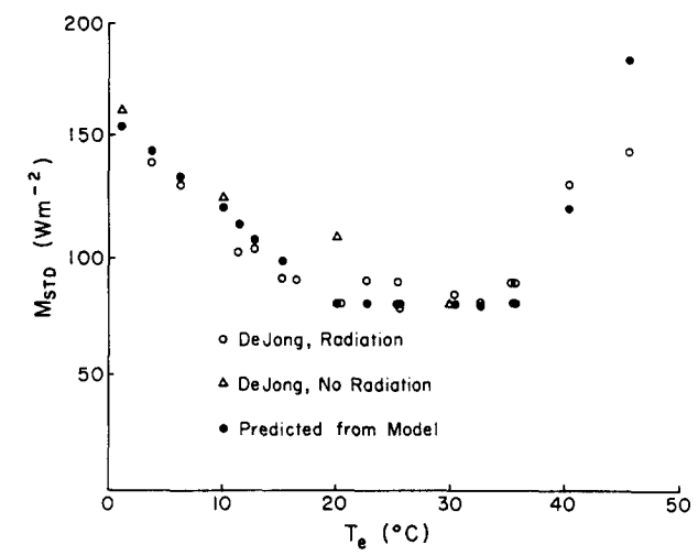
$Measured and predicted metabolic rates in relation to equivalent temperature ($T_e$). Estimates of metabolic rates ($M_{std}$) are based on each $T_e$ computed from the experimental conditions of DeJong (1976) applied to data on oxygen consumption in white-crowned sparrows reported by King (1964). These predictions (blackened circles) are compared with rates ($M_{std}$) actually measured by DeJong (1976) without added short-wave radiation (triangles) and with various intensities of short-wave radiation (unblackened circles). (From Mahoney, S.A. and J.R. King 1977, p. 118.).$

Figure 10.6: Measured and predicted metabolic rates in relation to equivalent temperature ($T_e$). Estimates of metabolic rates ($M_{std}$) are based on each $T_e$ computed from the experimental conditions of DeJong (1976) applied to data on oxygen consumption in white-crowned sparrows reported by King (1964). These predictions (blackened circles) are compared with rates ($M_{std}$) actually measured by DeJong (1976) without added short-wave radiation (triangles) and with various intensities of short-wave radiation (unblackened circles). (From Mahoney, S.A. and J.R. King 1977, p. 118.).

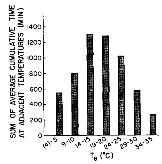
Equivalent temperature preferenda of white-crowned sparrows (mean values for four birds, each tested while alone in the preference apparatus). (From Mahoney, S.A. and J.R. King 1977, p. 199.)

Figure 10.7: Equivalent temperature preferenda of white-crowned sparrows (mean values for four birds, each tested while alone in the preference apparatus). (From Mahoney, S.A. and J.R. King 1977, p. 199.)

$Metabolic rate, $M$, of white-crowned sparrows, plotted as a function of standard operative temperature, $T_{es}$, for three different experiments, The solid line is the regression to the data in King (1964), This study used free convection in a darkened chamber. These conditions impose the least physiological stress, and gives the lowest standard metabolic rate in the thermoneutral zone.The birds were summer acclimated, giving a lower critical temperature of about $23^{\circ}C$, The solid symbols are the results of the study of Robinson et al. (1976), which used forced convection in a darkened chamber, Ran noise produces a slight (average of 11 percent) increase in 14 over King's (1.964) values. Data does not appear to extend into the thermoneutral zone. The open symbols are from DeJong's (1976) study, conducted using free convection in a chamber with various levels of visible radiation, The use of illuminated birds in the active part of their diurnal cycle gives the highest values of $M$. As these birds are winter-acclimated, the lower critical temperature is around $20^{\circ}C$. Note that the use of standard operative temperature allows the comparison of purely physiological differences under equivalent thermal conditions for different combinations of wind, radiation and air temperature.$

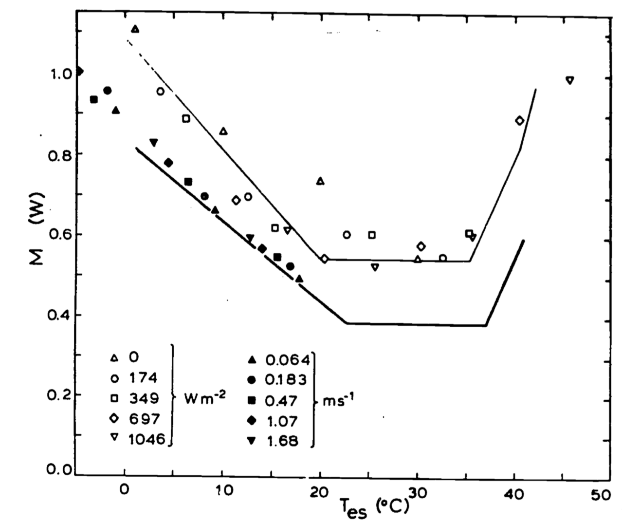
Figure 10.8: Metabolic rate, $M$, of white-crowned sparrows, plotted as a function of standard operative temperature, $T_{es}$, for three different experiments, The solid line is the regression to the data in King (1964), This study used free convection in a darkened chamber. These conditions impose the least physiological stress, and gives the lowest standard metabolic rate in the thermoneutral zone.The birds were summer acclimated, giving a lower critical temperature of about $23^{\circ}C$, The solid symbols are the results of the study of Robinson et al. (1976), which used forced convection in a darkened chamber, Ran noise produces a slight (average of 11 percent) increase in 14 over King’s (1.964) values. Data does not appear to extend into the thermoneutral zone. The open symbols are from DeJong’s (1976) study, conducted using free convection in a chamber with various levels of visible radiation, The use of illuminated birds in the active part of their diurnal cycle gives the highest values of $M$. As these birds are winter-acclimated, the lower critical temperature is around $20^{\circ}C$. Note that the use of standard operative temperature allows the comparison of purely physiological differences under equivalent thermal conditions for different combinations of wind, radiation and air temperature.

A second laboratory application of the $T_e$ concept is given by Bakken (1976b). He has elaborated on the measurement of equilibrium body temperature and thermal conductance of the body. Previously, Newton’s law of cooling has been used to describe the change in body temperature (but see Calder 1972, Kleiber 1975).

\[\begin{equation} \frac{d T_b}{dt} = \frac{K_n}{C} (T_b - T_a) \tag{10.6} \end{equation}\] where

$T_b$ is body temperature ($^{\circ}C$)
$T_a$ is air temperature ($^{\circ}C$)
$K_n$ is thermal conductance of body tissue ($J s^{-1}$)
$C$ is the heat capacity of the animal ($J$)
$t$ is time ($s$).

Equation (10.6) says that the change in body temperature will be zero when the animal’s temperature is equal to that of the air. This is not a bad approximation if $T_a = T_e$ and if the metabolic and water loss rates of the animal are small. Bakken (1976a) has shown that a better approximation of the cooling curve is given by

\[\begin{equation} \frac{d T_b}{dt} = \frac{K_0}{C} (T_b - (T_e + \frac{M-E}{K_0})) \tag{10.7} \end{equation}\] When $\frac{d T_b}{dt} = 0$,

\[T_b = T_e + \frac{M-E}{K_0}\]

If the cutaneous water loss is small than equation (10.7) has the same form as the steady-state equation (10.5) developed earlier, where \[\begin{equation} T_e = \frac{h_c T_a + Q_n}{h_c + R} \tag{10.8} \end{equation}\] and \[\begin{equation} K_0 = \frac{K (h_c + R)}{K + h_c + R} \tag{10.9} \end{equation}\] $K_0$ is a function of the convection coefficient, $h_c$, which depends specifically on wind speed, a physical characteristic of the environment. Bakken (1976b) has provided a detailed discussion of the use of equation (10.6). As an illustration, consider the case when $M$ and $E$ are small (most insects and lizards). Then equation (10.7) reduces to

\[\begin{equation} \frac{d T_b}{dt} = \frac{- K_0}{C} (T_b - T_e) \tag{10.10} \end{equation}\] If wind speed and orientation are constant, the only physiological characteristic of the organism that would make it different from that of an inanimate object is its ability to regulate blood flow. (As an example, see Fig. 10.9.)

10.4.3 Field Applications

A particularly interesting application of the $T_e$ concept will be in field studies. Bakken and Gates (1975) and Bakken (1976) have reviewed the possibility of making model organisms with the same thermal properties as the animal under study. Using the models, one could map the temporal and spatial variation of the thermal environment. Once the models have been checked in laboratory situations, it will be much easier to take one temperature than to make the many microclimatological measurements necessary to compute the energy budget. Buttemer (1979) is the first to use this method. These measurements include longwave and shortwave radiation, air temperature, wind speed, wind direction and relative humidity. With this map in hand, it will be easy to see if the animal is selective in how it uses the environment. For example, one could ask: is the laboratory behavior found in the sparrows studied by Mahoney and King (1977) exhibited out of doors? The $T_e$ concept is a straightforward method for tackling this kind of problem.

What would such a map look like? Data presented by Bakken and Gates (1975) in Table 10.2 gives some insight. The authors investigated the effect of absorptivity (points 1-3), orientation (3-5), microhabitat (3, 6-8) and size (9-13).

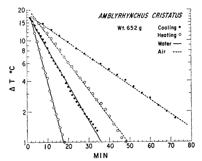
$Heating and cooling rates of the Galgpagos marine iguana (*Amblyrhynchus cristatus*) in water and air. $\Delta T$ is the difference between body and ambient temperatures ($T_a$). During heating $T_a = 40^{\circ}C$; during cooling $T_a=20^{\circ}C$. (From-G.A. Bartholomew and R.C. Lasiewski, 1965, Comp. Biochem. Phsio14-16173-582.)$

Figure 10.9: Heating and cooling rates of the Galgpagos marine iguana (Amblyrhynchus cristatus) in water and air. $\Delta T$ is the difference between body and ambient temperatures ($T_a$). During heating $T_a = 40^{\circ}C$; during cooling $T_a=20^{\circ}C$. (From-G.A. Bartholomew and R.C. Lasiewski, 1965, Comp. Biochem. Phsio14-16173-582.)

This approach will allow one to answer the question of whether or not animals avoid stressful environments. And what proportion of their time is spent in non equilibrium, requiring the organism to monitor its heating and cooling rates? Operative environmental temperature distributions combined with physiological measures of animals in the natural environment will give a better understanding of the influences of the thermal environment. An interesting example of such measurements is the body temperature telemetry taken from Pearson and Bradford (1976), who studied the thermoregulation of the lizard Liolaemus multicarpus and the toad Bufo spinulosus high in the Andes mountains. Figure 10.10 shows a record of the body temperature of both animals as a function of time. Although in similar microhabitats, each species interacts with the environment quite differently, which is manifested in their different body temperatures and activity patterns.