14.5 Theories of Turbulence
Businger (1973) states that “the primary objective of the study of turbulence in the atmospheric boundary layer is to obtain tractable expressions for the fluxes of heat, momentum, water vapor and other atmospheric constituents.” This is true not only for large scale interactions of, for example, weather systems with the earth’s surface, but also on smaller scales, such as the heat balance of exposed animals or the carbon dioxide exchange of a plant leaf. We are of course not limited to atmospheric flows. Turbulent fluxes are also important in the marine or aquatic environment, where we might include such things as nutrient fluxes, or the “fluxes” of the organisms themselves, borne about by the currents. An interesting example of this latter phenomenon is the formation of cold-core rings, which are giant eddies which break off from large meanders of the Gulf Stream (Wieke, 1976). Ranging up to 300 kilometers in horizontal extent, these eddies form around a “core” of seawater of different origin, and persist for up to two years. Consequently, they are of great ecological importance, since they represent a large scale intrusion of one oceanic community by another (the one surrounded by the eddy). It is thought that a better understanding of the factors which ultimately limit the distribution of oceanic, planktonic organisms may be gained by study of such structures.
Despite the importance of the study of turbulence for the various types of flow encountered in nature, in most cases rigorous analytic solutions do not yet exist. The equations of motion previously referred to should in theory describe turbulent flow in detail, but the extreme nonlinearity of the equations plus the randomness of turbulent flows makes this approach unfeasible at present. Consequently, most theories of turbulence are semi-empirical in nature. That is, they are based on a theoretically sound base, such as the Navier-Stokes (N-S) equations, but also rely on empirical assumptions about the processes involved to complete the theory. In short, unlike the case in many other physical theories, the equations do not tell the whole story of turbulence. Rather, the key to success appears to be the inventiveness of the researcher in applying the crucial simplifying assumptions. This is the problem and challenge of turbulence research.
It is due primarily to this very inventiveness that the uninitiated often find themselves awash in a sea of seemingly ad hoc assumptions and oversimplifications if they should attempt to read the turbulence literature. But, as in much scientific writing, a certain level of prior knowledge of the subject is usually assumed. While a thorough understanding of this “background material” is appropriate to textbooks on the subject, this paper attempts to deal with some of the most common material. Since we are primarily interested in calculating fluxes, it is appropriate that this final section deal with flux estimating procedures, drawing upon prior developments in this paper to link the procedure to the theory and phenomenon of turbulence.
14.5.1 Reynolds Averaging
Most semi-empirical theories are based upon a set of equations derived from the N-S equations called the Reynolds equations. The derivation is straightforward, and involves dividing the motion into its mean and fluctuating parts (see Cowan 1979a or Tennekes and Lumley 1972). The variables of interest are the pressure and the three velocity components. As an example, consider the decomposition of the velocity in the x-direction, \[u = \bar u + u'\] The overbar refers to the time average in the case of steady flow (see Cowan 1979a or Vennard and Street 1975), and the prime refers to the fluctuation around the mean (Fig. 14.7).
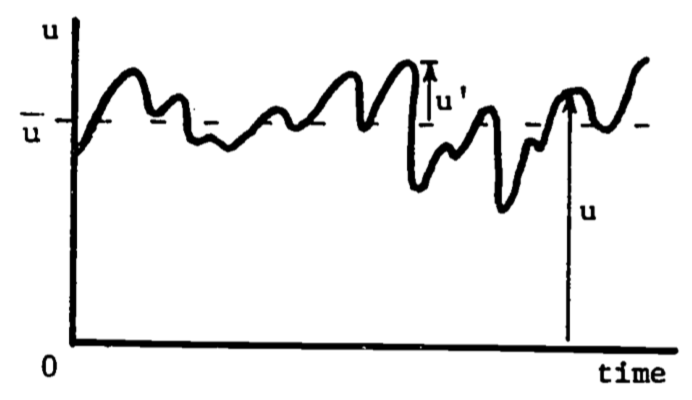
Figure 14.7: Velocity components–fluctuations around the mean.
The four expressions so derived are substituted into the N-S equations, and the resultant equations are then averaged over time, producing the Reynolds equations. This process is called Reynolds averaging, and it removes the rapidly varying nature of the N-S equations, at the expense of the addition of other terms. The net result is to introduce more unknowns (through the additional terms) than there are equations, making unique analytical solutions impossible. This so-called closure problem of turbulence is what leads to the necessity of introducing empirical equations for the extra unknowns, as was discussed earlier. Investigations of such empirical methods comprise a major part of the study of turbulence.
As a practical example of this, let us consider flow in the atmospheric surface layer. Assume that the mean wind (\(\bar u\)) is in the x-direction, and write the resultant simplified Reynolds equation for the x-component (Tennekes and Lumley 1972, p. 30ff).
\[\begin{equation} \frac{d \overline u}{dt} = - \frac{1}{\rho}\frac{d \overline P}{dx} + \frac{\partial}{\partial z} \bigg(- \overline{u'w'} + \frac{\mu}{\rho} \frac{\partial \overline u}{\partial z} \bigg) \tag{14.3} \end{equation}\]
Here \(\rho\) is air density (assumed constant), \(\overline P\) is wean air pressure, \(w\) is vertical velocity, and \(\mu\) is air viscosity (also assumed constant). Each term has the units of acceleration. The first term on the right represents acceleration due to pressure gradients. The first term in brackets is the “additional” term introduced by Reynolds averaging, and it represents acceleration due to turbulent shear stresses (see the section on Turbulent Shear Flow). The last term in brackets accounts for acceleration due to viscous (laminar) shear stress, which, as may be surmised from earlier discussion, is negligible compared to turbulent shear stress (except right at the surface, in the laminar boundary layer). We recognize that, using equation (14.3), we could rewrite the bracketed portion of equation (14.4) as
\[\begin{equation} - \frac{1}{\rho} \rho \overline{u'w'} + \frac{1}{\rho} \tau \tag{14.4} \end{equation}\]
One would then be tempted (if they were also a turbulence researcher!) to assume that the first term also represents a stress \(\tau_t\), possibly due to the turbulence (\(\tau_t\) is a subscripted stress and does not represent a time derivative.):
\[\begin{equation} \tau_t = -\rho \overline{u'w'} \tag{14.5} \end{equation}\]
In fact, it turns out that equation (14.5) does not represent the contribution of the turbulent motion to the mean stress. This was discussed in the section on Turbulent Shear Flow, but further development is warranted here.
An averaged product of fluctuating variables such as equation (14.5) is called a correlation. If the variables in such a product have the same (opposite) sign for most of the time as do \(a\) and \(b\) in Fig. 14.8, then the product is greater than (less than) zero. Notice that the variable \(c\), on the other hand, is uncorrelated with either \(a\) or \(b\), hence the products \(\overline{ac}\) or \(\overline{be}\) probably equal zero. In terms of \(u'\) and \(w'\), this means that if the vertical wind fluctuations are positive (upward) when the horizontal wind fluctuations are negative, and vice versa, then \(u'\) and \(w'\) are negatively correlated, hence the minus sign in equation (14.5). Such an interpretation also agrees with the turbulent velocity profile in Fig. 14.6 and the subsequent discussion. Momentum is constantly being transported downward (or momentum deficit is being transported upward). The end result is that the surface absorbs momentum from the flow, and consequently experiences a frictional force acting in the direction of the flow. As required by Newton’s Third Law, this force is opposed by frictional drag exerted on the air by the surface.
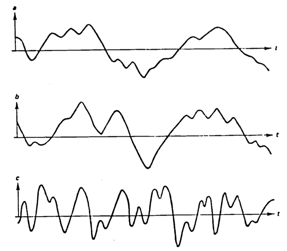
Figure 14.8: Variables and b are corelated (adapted from Tenekes and Lumley 1972).
In practice, expressions such as equation (14.5) are used in the actual measurement of surface fluxes in the atmosphere. It has been found that the fluctuating horizontal velocity term (\(u'\)) can be replaced with the fluctuating component of virtually any trace constituent (such as water vapor or CO2), thus obtaining the flux of that quantity. However, an emphasis on obtaining the maximum amount of information with the minimum amount of measurement precludes use of this correlation technique in most biological applications at present. This is due to the fact that the quantities to be measured are generally varying quite rapidly, so that a measurement and multiplication must be accomplished up to ten times a second. The next section introduces a more common general method of flux determination, which though simpler loses some of the insight into the actual physical processes which the correlation approach provides.
14.5.2 K Theory
Recall the discussion of the section titled Origins of Turbulence, in particular the similarities pointed out between turbulent and laminar shear stress. These similarities, in addition to the complexity of the equations of motion, make it tempting to write the expression for turbulent stress in a manner analogous to equation (14.3),
\[\begin{equation} \tau_t = \rho K \frac{d \overline u}{dy} \tag{14.6} \end{equation}\]
As the previous section demonstrated, such an assumption considerably simplifies the mathematics. In addition, it turns out that in many cases of substantial practical interest, such an approach has adequate predictive abilities. However, several objections can be raised to these so-called “K-theories”. First of all, it must be remembered that viscosity is a property of the fluid itself, depending basically upon its molecular makeup. Turbulence, and hence the “eddy viscosity” (\(K\)) in equation (14.6), are properties of the flow, and do not depend on the fluid. A perhaps more subtle distinction is that the time and length scales of turbulent flow are generally of the same order of magnitude as those scales representing the distribution of the property of interest, while the scales for molecular diffusion are much smaller. Thus the similarity of turbulent and molecular diffusion must be approached with caution (Lumley and Panfsky 1964). So while the adoption of a K theory formulation implies that the attempt to understand the turbulence has been de-emphasized; the success that K theories have enjoyed in certain useful applications have made them a valuable tool.
It is useful to again use the tool of dimensional analysis to extend the discussion of the section titled “Diffusivity” and derive a dimensional estimate for \(K\). Analogous to the development of equation (14.1), one may write a time scale for turbulent diffusion \((\tau_t)\) as \[T_t \sim \frac{L^2}{K_H}\] where \(K_H\) is the eddy diffusivity for heat analogous to \(\gamma\), the thermal diffusivity constant. It is reasonable to require that this time be of the same order as the characteristic time defined in equation (14.2). Thus we can write \[T_t \sim \frac{L}{K_H} \sim \frac{1}{U_c}\] which gives us the following expression for \(K_H\): \[\begin{equation} K_H \sim U_cL \tag{14.7} \end{equation}\] Diffusion type equations may be written for quantities besides heat, including mass and momentum. Hence expressions such as equation (14.7) are perfectly general, and one finds them frequently in applications.
Let us illustrate a common method of utilizing an expression like equation (14.7) in practical applications. The previous discussion of atmospheric turbulence suggests that the natural choice of a length scale for a wallbounded flow would be the distance from the surface to the measuring point, \(z\). Recall that this can be thought of as the size of the most efficient energy transporting eddy. \(u_*\), the so-called friction velocity, is the velocity scale used. It is defined by the expression \[\begin{equation} \tau = \rho u^2_* \tag{14.8} \end{equation}\] which can be easily shown to be correct dimensionally. Qualitatively, it can be thought of as the tangential rate of rotation of the eddies. In this way, it can be related to the expression for dynamic wind pressure in Bernoulli’s equation, \(1/2\rho u^2\) (see, e.g., Vennard and Street 1975). Also, there is the relation \[\begin{equation} K_M = ku_*z \tag{14.9} \end{equation}\] where \(K_M\) is the eddy transport coefficient of momentum of eddy viscosity and where \(k\) has been shown experimentally to be a constant, approximately equal to 0.4, and is known as von Karman’s’constant.
Normal practice in micrometeorology, for example, is to substitute equations (14.8) and (14.9) into the gradient relation (equation (14.6)) and solve for \(u_*\), \[\begin{equation} u_* = kz \frac{d \overline u}{dz} \tag{14.10} \end{equation}\] This of course is tantamount to finding \(\tau\). \(u_*\) is important in certain mean gradient methods for finding the fluxes of heat and mass, notably the aerodynamic method (see, e.g., Campbell 1977 or Monteith 1973 or 1975) and the combination or Penman type methods. A particularly lucid exposition of these methods as applied to evapotranspiration can be found in Chapter 3 of Taylor and Ashcroft (1972). It should be apparent from the one-dimensional nature of equations (14.6), (14.9) and (14.10) that we are considering transport to be occurring in only one direction, normal to the surface. This is the case when we consider flow over an essentially infinitely long, horizontal and homogeneous surface. Transport to or from small objects such as animals requires a different approach.
14.5.3 Boundary Layers and Non-dimensional Numbers: A Bulk Approach
Implicit in the present treatment of turbulence has been the proximity of a surface to the flow. As discussed previously, much turbulence originates at surfaces. Out of the main sources of turbulence is the friction between the fluid and the surface (mechanical turbulence). Another important source is due to heating of the surface, which transfers heat to the fluid, causing the less dense, heated fluid to rise (thermal turbulence). If there is bulk movement of the fluid, mechanical turbulence is present, but of course only in the area where the frictional influence of the surface is important. This region of surface influence is known as the boundary layer. It can be characterized by a boundary layer depth, which corresponds to the streamline along which the velocity reaches 99% of the free stream velocity (see Fig. 14.9). This latter velocity is the one which characterizes the fluid away from the retarding influence of the surface. Notice in Fig. 14.9 that the flow is initially laminar, changing to turbulent, with a transition region of mixed laminar and turbulent flow called the viscous sublayer. This flow structure is due primarily to the fact that the fluid layer immediately next to a surface has zero velocity with respect to the surface, and the flow must adjust itself accordingly. See Vennard and Street (1975) or Monteith (1930) for a further discussion of boundary layers.
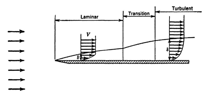
Figure 14.9: Visualization of the development of the boundary layer velocity profile. From left to right, the initial uniform velocity shows a laminar profile upon first contact with the surface. This develops into a turbulent layer if the Reynolds number is large. From Vennard and Street 1975, p. 312.
K theory, or the gradient approach, requires measurements to be taken in the boundary layer region, an approach especially suitable where the boundary layer is extensive, such as in wind flow over the earth’s surface. However, measurements within the boundary layer become extremely difficult around small objects, such as animals or leaves. Due to the complex geometry, small size and many possible orientations with respect to the wind for such objects, it becomes practically impossible to define where the boundary layer is, let alone take measurements there. Consequently, in the case of small objects, a bulk approach is taken. Measurements of the property being transported are taken in the environment, far enough away so that the surface does not influence the flow, and at the surface itself. This approach is practical here because for small objects the boundary layer is sufficiently thin for this difference in properties to be clearly defined.
The bulk approach is actually an integrated form of the gradient approach (Businger 1973) and thus is still based on the same molecular analogy. Taking heat transfer as an example, one may write the flux of heat (\(F_H\)) for a still fluid as \[\begin{equation} F_H = \frac{k}{\delta} (T_0 - T_\infty) \tag{14.11} \end{equation}\] where \(k\) is the thermal conductivity of the fluid, \(\delta\) is the uniform boundary layer depth, and \((T_0 - T_\infty)\). is the difference between surface and environmental temperatures, respectively. Equation (14.11), as presented, is exact in its description. In the more general case, where the fluid can be in motion, the boundary layer may be turbulent and of variable depth and structure. In this case, \(\gamma\) becomes a sort of average or equivalent boundary layer depth, not directly measurable. An empirical approach has been proposed (Monteith 1973) which is well borne out by experiment. First, write equation (14.11) as \[\begin{equation} F_H = (\frac{d}{\delta}) \frac{k}{d} (T_0 - T_\infty) \tag{14.12} \end{equation}\] were \(d\) is a characteristic length (e.g. the diameter of a sphere or cylinder, the length of a flat plate in the direction of flow). Then rearrange equation (14.12) \[\begin{equation} Nu = \frac{d}{\delta} = \frac{F_H}{(k/d)(T_0 - T_\infty)} \tag{14.13} \end{equation}\] This is the defining relation for the Nusselt number (\(Nu\)). When determining the heat flux, equation (14.11) would normally be written \[\begin{equation} F_H = Nu(k/d)(T_0 - T_\infty) \tag{14.14} \end{equation}\] Notice that all quantities on the right-hand side of equation (14.14) are directly available except \(Nu\). If equation (14.14) is to be of any more practical use than equation (14.11), a means of determining \(Nu\) is required.
Equation (14.13) points in the general direction of the method used to find \(Nu\). It can be regarded as a purely empirical constant, and under suitable conditions \(F_H\) and \(k/d(T_o - T_\infty)\) can be determined independently for different conditions of flow and geometry, and its values tabulated. It turns out that for a given geometry and orientation to the flow, \(Nu\) can be written \[\begin{equation} Nu = A Re^n \tag{14.15} \end{equation}\] for forced convection. Thus, once \(A\) and \(n\) are determined for a particular geometry and orientation, \(Nu\) is calculable. This should not be surprising, since \(Re\) is an indicator of turbulence, and it has been demonstrated that \(Nu\), an indicator of heat transfer, is a function of the degree of turbulence. Notice also that equation (14.15), by use of \(Re\) instead of just the velocity, has taken into account the effects of fluid viscosity and characteristic length of the body, making \(A\) and \(n\) independent of body size.
This dependence of \(Nu\) on \(Re\) indicates that \(Nu\) is not “purely empirical.” Consider the ratio in the defining relation of equation (14.13), \(F_H/\frac{k}{d}(T_0 - T_\infty)\). This can be thought of as the ratio of actual heat flux (\(F_H\)) to that which would result in a stationary fluid layer of depth \(d\) due to the same temperature difference (\(T_0 - T_\infty\)). Thus, for a still fluid layer over a flat plate, we would expect \(Nu=1\). Heat transfer is of course more efficient in a flowing fluid, especially, as discussed earlier, if the flow is turbulent. Therefore we would expect \(Nu>1\) in these cases. \(Nu\) is also a function of geometry. For example, \(Nu=2\) for a sphere in a still fluid (see Businger 1973, p.68 for a derivation). In practice, then, we find different geometries (and orientations) treated separately. Note, however, in Fig. 14.11, that geometry is not extremely critical, e.g. a man and a sheep behave essentially as cylinders. Another nondimensional number, the Grashof number (\(Gr\)), assumes the place of \(Re\) for the free convection case.
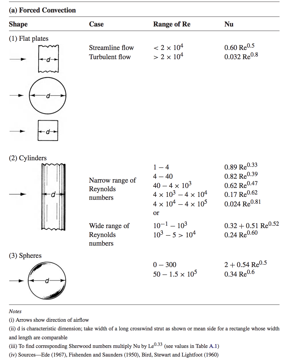
Figure 14.10: Nusselt numbers for air: forced convection From Monteith 1973, p. 224.
A convenient tabulation of various dimensionless numbers is in Campbell (1977, p.65). Monteith (1973, pp.224-225) tabulates \(Nu\) for forced and free convection, various geometries, and ranges of \(Re\) (or \(Gr\)). Part of this table is reproduced in Fig. 14.1. Using the information there, in conjunction with equation (14.14), one can obtain estimates of heat flux for various body geometries, wind speeds, and body size. The quantity \(Nu \frac{k}{d}\) is related to similar terms used by various authors such as the heat transfer coefficient (\(h\)) and the exchange resistance (\(r\)) by the expression \[ Nu \frac{k}{d} = h = \frac{\rho c_p}{r}\] where \(\rho\) is fluid density and \(c_p\) is specific heat.
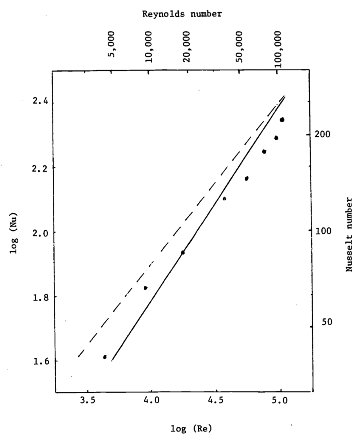
Figure 14.11: A plot ofthe Nusselt number versus the Reynolds number compares convective heat transfer from a man (- -) and a sheep (\(\cdots\)). The data are fairly close to theoretical calculations made for a cylinder (—). From Monteith 1972, p. 111.