7.5 Examples of Heat Energy Budget

To illustrate the heat transfer principles and their biological importance, we chose three systems: the soil, a leaf, and a lizard. Again, the reader is asked to think of the ecological importance of the system and how the thermal balance influences physiological processes as the examples are presented.

7.5.1 Heat Flow in Soil

In soil, heat flow has great biological importance. Not only does the energy balance control the soil temperature, but it greatly affects the moisture content. Both factors are important for photosynthesis in green plants. Soil temperature also influences nutrient uptake as we have seen in our example at the beginning of the module. Fungi, bacteria, insects, as well as many other invertebrates and vertebrates, commonly spend part or all of their life cycles in or surrounded by the soil. Soil temperatures influence metabolic rates and may serve as a behavioral cue for daily and seasonal activity patterns.

The simplest representation of heat flow in the soil is a conduction process where the heat flux $dQ$ per unit time $dt$ is equal to the conductivity $k$ times the difference in temperature $dT$ over a unit path length $dz$. \[\begin{equation} \frac{dQ}{dt} = -k \frac{dT}{dz} \tag{7.21} \end{equation}\] The minus sign is used to indicate that the potential gradient is in the direction of decreasing temperature.

Another result can be derived by considering Fig. 7.7. The First Law states that the change in internal energy (storage) is equal to the inflow minus the outflow. The change in internal energy will be equal to the mass ($\rho d z$) times the heat capacity ($c$), multiplied by the change in temperature with time ($\Delta T$).

\[\begin{align} c \rho \Delta T \, d z &= k \bigg(\frac{dT}{dz}\bigg)_U - k \bigg(\frac{dT}{dz}\bigg)_L \notag \\ \Delta T &= \frac{k}{c\rho} \frac{1}{dz} \Bigg( \bigg(\frac{dT}{dz}\bigg)_U - \bigg(\frac{dT}{dz}\bigg)_L\Bigg) \notag \\ \frac{\partial T}{\partial t} &= \frac{k}{c \rho} \frac{\partial^2 T}{\partial z^2} \tag{7.22} \end{align}\] Equation (7.22) is a form of the diffusion equation and $\frac{k}{c \rho}$ is called the thermal diffusivity. This equation can be solved analytically if simple enough boundary conditions are assumed and the thermal diffusivity remains constant. In general, the diffusivity is a function of the water content of the soil and the soil temperature (here numerical methods must be used). We can, however, get a feeling for the heat transfer profile by noting the general boundary conditions. We know that at the soil surface under steady state conditions the temperature will cycle daily while at some depth $z_0$ below the surface the temperature will not change.

Figures 7.8 and 7.9 from Lowry (1969) give different representations of how the soil might change with time and depth. Simpson (1977), Carslaw and Jaeger (1959), and Van Wijk (1966) present a more detailed discussion of soil heat flow.

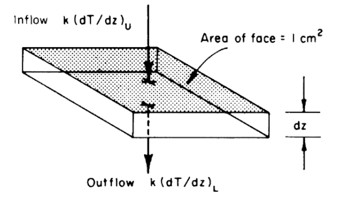
Schematic view of a unit of soil, showing heat inflow from above and heat outflow below, leading to derivation of Eq. 7.22. (From Lowry, W.P. 1969. P. 51)

Figure 7.7: Schematic view of a unit of soil, showing heat inflow from above and heat outflow below, leading to derivation of Eq. 7.22. (From Lowry, W.P. 1969. P. 51)

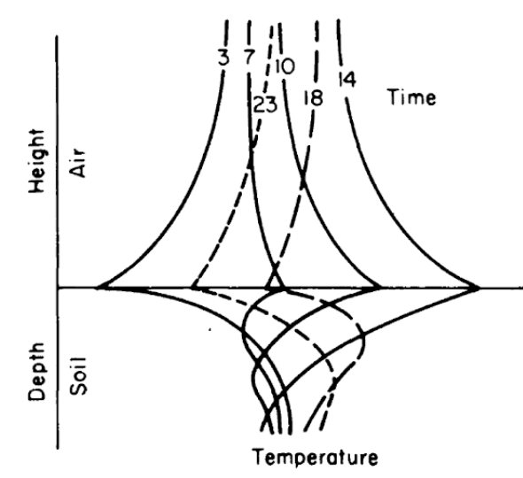
Generalized soil-air temperature profiles (tautochrones) near the soil surface, for four-hour intervals during a diurnal period. (From Lowry, W.P. 1969. P.37.)

Figure 7.8: Generalized soil-air temperature profiles (tautochrones) near the soil surface, for four-hour intervals during a diurnal period. (From Lowry, W.P. 1969. P.37.)

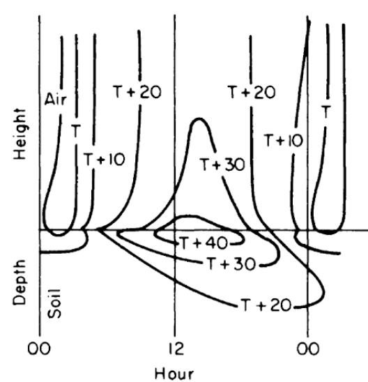
Figure 7.9: Generalized diurnal patterns of isotherms near the soil surface on coordinates of time and distance. (From Lowry, W.P. 1969. P. 37.)

7.5.2 A Leaf

Our second example is the energy balance of a leaf. Gates (1968) chose to model the heat balance of a leaf because it has a distinct physical geometry and because it is the unit of photosynthesis. The governing heat flux equation for the steady state condition was given in the module on the First Law of Thermodynamics and is repeated here:

\[\begin{equation} Q_a = Q_e + C + LE \tag{7.23} \end{equation}\] where

$Q_a$ is the radiant energy absorbed by the leaf ($W m^{-2}$),
$Q_e$ is the energy emitted by the leaf ($W m^{-2}$),
$C$ is the convective flux ($W m^{-2}$), and
$LE$ is the evaporative flux ($W m^{-2}$).

With empirical measurements and some assumptions (see Gates 1977), equation (7.23) is expanded as: \[\begin{equation} Q_a = \varepsilon \sigma (T_l + 273)^4 + k_1 \bigg(\frac{V}{D}\bigg)^{0.5} (T_l - T_a) + L (T_l) \frac{_s d_l (T_l) - [r.h.]_s d_a (T_a)}{r_l + k_2 (D^{0.3} W^{0.20}) / V^{0.50}} \tag{7.24} \end{equation}\] where

$\sigma$ is the Stefan-Boltzmanm constant ($5.67 \times 10^{-8} W m^{-2} K^{-4}$)
$\varepsilon$ is the emissivity of the leaf
$T_l$ is the leaf temperature ($^{\circ}C$),
$V$ is the wind speed ($m s^{-l}$),
$k_1$ is an experimentally determined coefficient ($9.14 J m^{-2} s^{-0.5} {^{\circ}C^{-1}}$),
$k_2$ is an experimentally determined coefficient ($183 s^{0.5} m^{-1}$),
$T_a$ is the air temperature ($^{\circ}C$),
$D$ is the leaf dimension in the direction of the wind ($m$),
$r.h.$ is the relative humidity,
$W$ is the leaf dimension transverse to the wind (m),
$_s d_l (T_l)$ is the concentration of water vapor saturation at leaf temperature $T_l (kg \, m^{-1})$,
$_s d_a (T_a)$ is the concentration of water vapor in free air saturated at air temperature $T_a (kg \, m^{-1})$, and
$r_l$ is the internal diffusion resistance of the leaf ($s m^{-1}$).

Inspection of equation (7.24) shows that the energy balance of the leaf is very dependent on leaf temperature which in turn affects convection and transpiration. To analyze this multivariate problem, Gates graphed three variables while holding the rest constant. Figures 7.10 and 7.11 illustrate thermodynamic conditions that would be common in tropical habitats at midday sunny ($Q_a = 900 W m^{-2}$) and cloudy ($Q_a = 600 W m^{-2}$) radiation levels. Note the differences in transpiration rates and leaf temperatures as a function of leaf resistance. Gates (1968) also considered the effects of leaf size. Figure 7.12 clearly shows that small leaves, by reducing leaf temperature and transpiration, would be advantageous in desert regions.

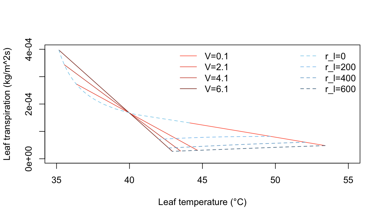
Computed transpiration rate versus leaf temperature as a function of wind speed and internal diffusive resistance for the conditions indicated. (From Gates, D. M. 1968. P. 216.)

Figure 7.10: Computed transpiration rate versus leaf temperature as a function of wind speed and internal diffusive resistance for the conditions indicated. (From Gates, D. M. 1968. P. 216.)

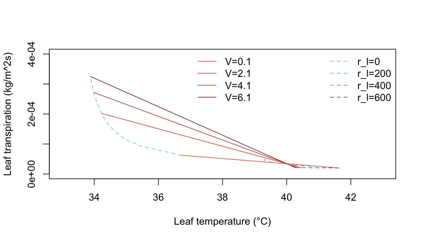
Figure 7.11: Computed transpiration rate versus leaf temperature as a function of wind speed and internal diffusive resistance for the conditions indicated. (From Gates, D. M. 1968. P. 217.)

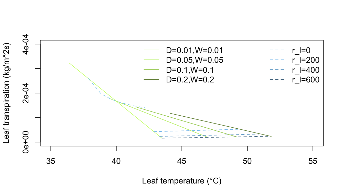
Computed transpiration rate versus leaf temperature for various leaf dimensions and internal diffusive resistances for the conditions indicated. (From Gates, D. M. 1968. P. 229.)

Figure 7.12: Computed transpiration rate versus leaf temperature for various leaf dimensions and internal diffusive resistances for the conditions indicated. (From Gates, D. M. 1968. P. 229.)

7.5.3 A Lizard

As a final example, we will review the work of Bartlett and Gates (1967) who computed the heat energy budget for the Western fence lizard, Sceloporus occidentalis, on a tree trunk. They hypothesized that S. occidentalis oriented itself on the tree trunk so as to maintain its body temperature relatively high and constant. The daily temperature variation of the tree surfaces supported their idea (Fig. 7.13). The heat energy equation for equilibrium is

\[\begin{equation} Q_a + M - Q_e - LE - C - G = 0 \tag{7.25} \end{equation}\] where

$Q_a$ is energy absorbed ($W m^{-2}$),
$M$ is metabolism ($W m^{-2}$),
$Q_e$ is radiation emitted ($W m^{-2}$),
$LE$ is evaporation ($W m^{-2}$),
$C$ is convection ($W m^{-2}$), and
$G$ is conduction ($W m^{-2}$).

Equation (7.25) may be rewritten:

\[\begin{equation} Q_a + M - \varepsilon \sigma A_e (273 + T_s)^4 - LE - h_c A_c (T_s - T_a) - k A_c \frac{dT}{dx} = 0 \tag{7.26} \end{equation}\]

where

$\varepsilon$ is emissivity to longwave radiation,
$\sigma$ is Stefan-Boltzmann constant ($5.67 \times 10^{-8} W m^{-2} K^{-4}$),
$A_e$ is the percent of the total surface area of the animal not in contact with substratum,
$T_s$ is surface temperature of the lizard ($^{\circ}C$),
$h_c$ is convection coefficient ($W m^{-2} {^{\circ}C^{-1}}$),
$T_a$ is air temperature ($^{\circ}C$),
$k$ is thermal conductivity of substratum ($W m^{-1} {^{\circ}C^{-1}}$),
$A_c$ is the percent area of the animal total surface area in contact with the substratum,
$\frac{dT}{dx}$ is temperature gradient with the substrate ($^{\circ}C m^{-1}$).

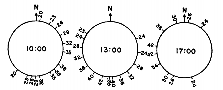
$Tree surface temperature in $^{\circ}C$ on Chew's Ridge at 10:00, 1.:00, and 17:00 Pacific Standard Time June 21 as a function of direction from North. (From Bartlett, P. N. and D. M. Gates. 1967. P. 320.)$

Figure 7.13: Tree surface temperature in $^{\circ}C$ on Chew’s Ridge at 10:00, 1.:00, and 17:00 Pacific Standard Time June 21 as a function of direction from North. (From Bartlett, P. N. and D. M. Gates. 1967. P. 320.)

The terms of equation (7.26) were either experimentally determined or taken from the literature. It was then solved for a variety of situations to obtain a range of values for the animal’s energy balance:

A maximum heat gain: If the lizard’s surface temperature $T_s$ equaled 29.3 °C and the lizard was in close contact with the tree.
A minimum heat gain: If $T_s = 39.9 ^{\circ}C$ and the lizard was not in contact with the tree.
Maximum heat loss of $T_s = 38.9 ^{\circ}C$, wind speed = $2.23 m s^{-1}$ (5 mph) and the animal was oriented at $90^{\circ}$ to the direction of the wind.
Minimum heat loss if $T_s = 29.3 ^{\circ}C$, and wind speed was $0.1 m s^{-1}$.
Intermediate heat loss if $T_s = 34.1 ^{\circ}C$ and wind speed = $0.45 m s^{-1}$. Figure 7.14 gives sample results.

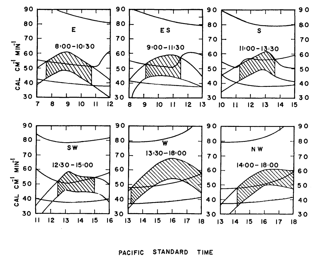
Max and min energy gains (concave downward) and maximum, minimum, and estimated energy losses (concave upward) of a lizard on a tree trunk on Chew's Ridge for selected times and positions on June 21, with times when lizards could be expected to be found at the selected positions. Areas hatched represent times when the estimated energy loss falls between maximum and minimum energy gains. (From Bartlett, P. N. and D. M. Gates. 1967. P. 321.)

Figure 7.14: Max and min energy gains (concave downward) and maximum, minimum, and estimated energy losses (concave upward) of a lizard on a tree trunk on Chew’s Ridge for selected times and positions on June 21, with times when lizards could be expected to be found at the selected positions. Areas hatched represent times when the estimated energy loss falls between maximum and minimum energy gains. (From Bartlett, P. N. and D. M. Gates. 1967. P. 321.)

Estimated hourly positions on a tree trunk on Chew's Ridge for June 21 where (*Sceloporus occidentalis* could maintain its characteristic body temperature (arrows) and actual observed positions of lizards on June 21, 1964 (crosses). (From Bartlett, P. N. and D. M. Gates. 1967. P.321.)

Figure 7.15: Estimated hourly positions on a tree trunk on Chew’s Ridge for June 21 where (Sceloporus occidentalis could maintain its characteristic body temperature (arrows) and actual observed positions of lizards on June 21, 1964 (crosses). (From Bartlett, P. N. and D. M. Gates. 1967. P.321.)

Finally, they calculated the energy losses and gains every hour at $45^{\circ}$ increments around the tree. Using the criterion that the energy losses must fall between the energy gains (Fig. 7.14), they could predict the position of the lizard on the tree trunk as a function of time of day. The predicted and observed positions of the lizards are compared in Fig. 7.15. TrenchR includes a Tb_lizard() function to model the energy balance of a lizard.

This module has attempted to develop the aspects of heat transfer that are important to biology. Emphasis has been placed on the physical processes, radiation, evaporation, conduction and convection, that influence the physiological, behavioral and ecological activities of all organisms. The discussion in conjunction with the modules on the First Law of Thermodynamics presents the basic physical laws that are needed to describe the heat energy balance of ecological systems.