7.3 Heat Transfer Processes
7.3.1 Radiation
Radiation is a process of energy transfer that requires no intervening medium. The dual nature of radiation, its particle (photon) and wavelike properties have important biological consequences. All matter radiates energy as individual photons (Kreith 1973) but for heat transfer problems the wavelike description is more useful. This is because energy at different wavelengths interacts with matter it different ways (see Problem 2). Figure 7.3 shows the different wavelengths of electromagnetic spectrum.
Since radiation travels at the speed of light \(c_L\), the product of the frequency \(f\) and the wavelength \(\lambda\) is a constant: \[\begin{equation} c_L = f \lambda \tag{7.1} \end{equation}\]
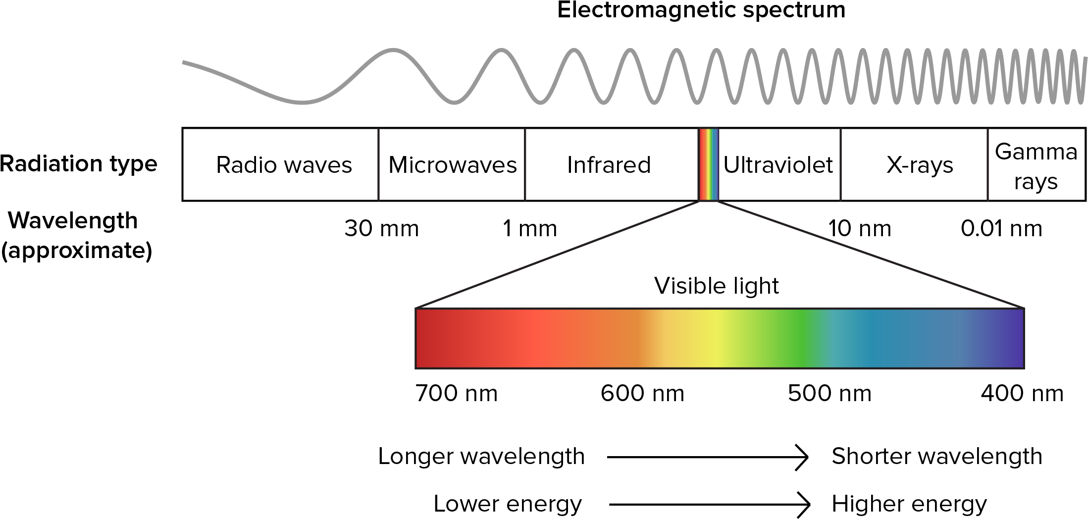
Figure 7.3: The electromagnetic spectrum.
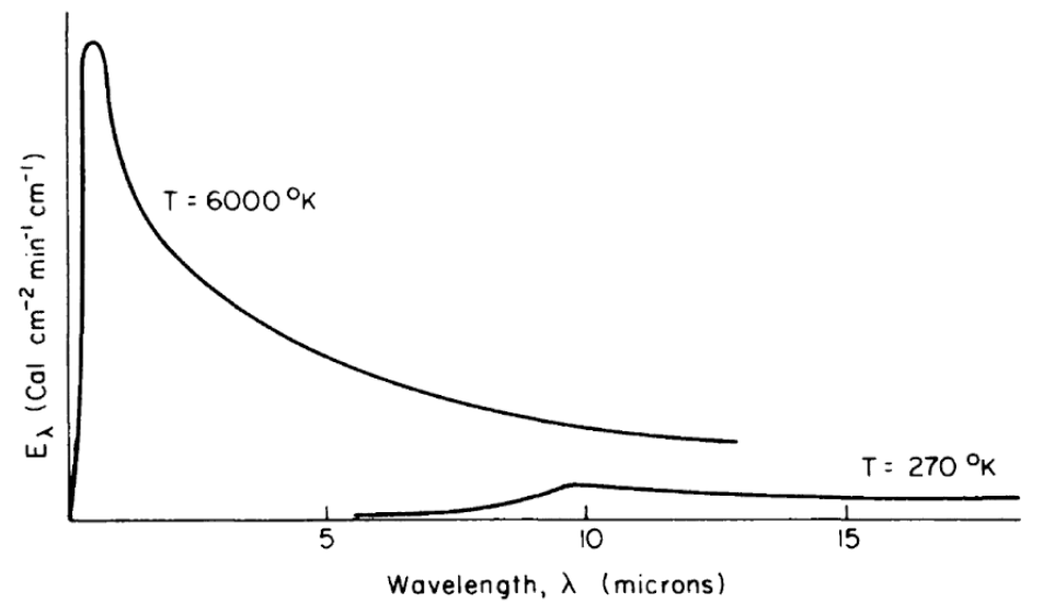
Figure 7.4: Schematic representation of blackbody emission spectra, as a function of wavelength, for temperatures of 6000 and 270 K. (From Lowry, W.P., 1969, p. 17.)
All objects, living and nonliving, radiate thermal energy. The amount and kind (wavelength in the electromagnetic spectrum) of energy depend on the temperature and physical characteristics of the radiating body. Figure 7.4 shows the energy radiated by the sun and the earth as a function of wavelength. It should be clear from the figure that the portion of the electromagnetic spectrum radiating from the sun occurs at much shorter wavelengths than that of the earth. In fact, the sun’s peak radiation on a wavelength plot is in the green part of the visible spectrum, while the earth’s radiation is completely in the infrared region.
Three physical laws are associated with figure 7.4. Planck’s Law gives the energy emitted, \(E_\lambda\), as a function of the wavelength, \(\lambda\), if the temperature of the radiating body is known: \[\begin{equation} E_\lambda = c_1 \lambda^{-5} [\exp(c_2 / \lambda T)] -1 ]^{-1} \tag{7.2} \end{equation}\] where- \(E_\lambda\) is the amount of energy emitted in the band \(\lambda\) to \(\lambda\) + \(d \lambda\) (\(J m^{-1}\)),
- \(T\) is the blackbody temperature (\(K\)),
- \(\lambda\) is the wavelength (\(m\)),
- \(c_1\) is \(2 \pi h {c_L}^2\),
- \(c_2\) is \(hc_L / K_b\),
- \(h\) is Planck’s constant = \(6.63 \times 10^{-34} (J s)\),
- \(K_b\) is Boltzmann’s constant = \(1.38 \times 10^{-23} (J K^{-1})\), and
- \(c_L\) is the speed of light = \(3.00 \times 10^8 (m s^{-1})\).
It is obvious that no one has actually measured the surface temperature of the sun. In this instance, the sun’s temperature was deduced from its electromagnetic spectrum. Second, from Planck’s Law, it can be demonstrated (Robinson 1966 or Roseman 1978) that the wavelength at the maximum radiated energy is only a function of the temperature of the radiating body.
\[\begin{equation} \lambda_{max} = \frac{2.897}{T} \times 10^{-3} \tag{7.3} \end{equation}\] where- \(\lambda_{max}\) = wavelength of maximum radiation (\(m\)), and
- \(T\) = temperature (\(K\)).
- \(Q_{emit}\) is the radiant energy emitted from the surface (\(W m^{-2}\)).
- \(\varepsilon\) is the emissivity (range zero to one),
- \(\sigma\) is the Stephan-Boltzmann constant (\(5.67 \times 10^{-8} W m^{-2} K^{-4}, 8.17 \times 10^{-11} cal \, min^{-l} cm^{-2} K^{-4})\), and
- \(T_s\) is the surface temperature (\(^{\circ}C\))
Roseman (1978) gives a more complete discussion of these laws.
Kirchoff studied the emissivity and absorptivity of materials. He showed that the energy absorbed at any specific wavelength \(\lambda\) at constant temperature is equal to the energy emitted at \(\lambda\). That is, if the absorptivity of a surface \(a(\lambda)\) represents the fraction of incident radiation absorbed at \(\lambda\) and \(\varepsilon (\lambda)\) is the emissivity, the radiation emitted at \(\lambda\) divided by the radiation emitted from a blackbody, then \(a(\lambda) = \varepsilon (\lambda)\) for each wavelength. If \(\varepsilon = 1\) for all wavelengths, then the object is said to be a blackbody. Although no system is a perfect blackbody, many are approximately so. In the infrared region, 3 to 100 \(\mu m\), most objects such as vegetation, soil and water behave like blackbodies (\(\varepsilon = 1\)). Table 7.1 gives the emissivities of some plants and animals.
Table 7.1. Long Wave Emissivities (percent, from Monteith, J.L., 1973, p. 68.)
Leaves
| Species | Average |
|---|---|
| Maize (Zea mays) | 94.4 ± 0.4 |
| Tobacco (Nicotiana tabacum) | 97.2 ± 0.6 |
| Snap bean (Phaseolus vulgaris) | 93.8 ± 0.8 |
| Cotton (Gossypium hirsutum Deltapine) | 96.4 ± 0.7 |
| Sugar cane (Saccharum officinarum) | 99.5 ± 0.4 |
| Poplar (Populus fremontii) | 97.7 ± 0.4 |
| Geranium (Pelargonium domesticum) | 99.2 ± 0.2 |
| Cactus (Opuntia rufida) | 97.7 ± 0.2 |
Animals
| Species | Dorsal | Ventral | Average |
|---|---|---|---|
| Red squirrel (Tamiasciurus hudsonicus) | 95-98 | 97-100 | |
| Gray squirrel (Sciurus carolinensis) | 99 | 99 | |
| Mole (Scalopus aquaticus) | 97 | – | |
| Deer mouse (Peromyscus sp.) | – | 94 | |
| Gray wolf | 99 | ||
| Caribou | 100 | ||
| Snowshoe hare | 99 | ||
| Man (Homo sapiens) | 98 |
Table 7.2. Reflectivities of Biological Materials for Solar Radiation (from Monteith, J.L., 1973, pp. 66-67.)
LEAVES Reflection coefficients r (%) for Solar Radiation
| Species | Upper | Lower | Average |
|---|---|---|---|
| Maize (Zea mays) | 29 | ||
| Tobacco (Nicotiana tabacum) | 29 | ||
| Cucumber (Cucumis sativa) | 31 | ||
| Tomato (Lycopersicon esculentum) | 28 | ||
| Birch (Betula alba) | 30 | 33 | 32 |
| Aspen (Populus tremuloides) | 32 | 36 | 34 |
| Oak (Quercus alba) | 28 | 33 | 30 |
| Elm (Ulmus rubra) | 24 | 31 | 28 |
VEGETATION – MAXIMUM GROUND COVER
| Farm Crops | Daily Mean | Farm Crops | Daily Mean |
|---|---|---|---|
| Grass | 24 | Wheat | 22 |
| Sugar beet | 26 | Pasture | 25 |
| Barley | 23 | Barley | 26 |
| Wheat | 26 | Pineapple | 15 |
| Beans | 24 | Sorghum | 20 |
| Maize | 18 - 22 | Sugar cane | 15 |
| Tobacco | 19 - 24 | Cotton | 21 |
| Cucumber | 26 | Groundnuts | 17 |
| Tomato | 23 |
| Natural Vegetation | Daily Mean | Natural Vegetation | Daily Mean |
|---|---|---|---|
| Heather | 14 | Natural pasture | 25 |
| Bracken | 24 | Derived savanna | 15 |
| Gorse | 18 | Guinea savanna | 19 |
| Maquis, evergreen scrub | 21 |
| Forests and Orchards | Daily Mean | Forests and Orchards | Daily Mean |
|---|---|---|---|
| Deciduous woodland | 18 | Eucalyptus | 19 |
| Coniferous woodland | 16 | Tropical rainforest | 13 |
| Orange orchard | 16 | Swamp forest | 12 |
| Aleppo pine | 17 |
ANIMAL COATS
| Mammals | Dorsal | Ventral | Average |
|---|---|---|---|
| Red squirrel (Tamiasciurus hudsonicus) | 27 | 22 | 25 |
| Gray squirrel (Sciurus carolinensis) | 22 | 39 | 31 |
| Field mouse (Microtus pennsylvanicus) | 11 | 17 | 14 |
| Shrew (Sorex sp.) | 19 | 26 | 23 |
| Mole (Scalopus aquaticus) | 19 | 19 | 19 |
| Gray fox (Urocyon cinereo argenteus) | 34 | ||
| Zulu cattle | 51 | ||
| Red Sussex cattle | 17 | ||
| Aberdeen Angus cattle | 11 | ||
| Sheep weathered fleece | 26 | ||
| Newly shorn fleece | 42 | ||
| Man (Homo sapiens) Eurasian | 35 | ||
| Negroid | 18 |
| Birds | Wing | Breast | Average |
|---|---|---|---|
| Cardinal (Richmondena cardinalis) | 23 | 40 | |
| Bluebird | 27 | 34 | |
| Tree swallow | 24 | 57 | |
| Magpie | 19 | 46 | |
| Canada goose | 15 | 35 | |
| Mallard duck | 24 | 36 | |
| Mourning dove | 30 | 39 | |
| Starling (Sturnus vulgaris) | 34 | ||
| Glaucous-winged gull (Larus glaucescens) | 52 |
This, however, is not true in the visible part of the spectrum. In general, any wavelength can be absorbed, reflected, or transmitted. This is written:
\[\begin{equation} a(\lambda) + r(\lambda) + t(\lambda) = 1 \tag{7.5} \end{equation}\]
where- \(a(\lambda)\) = absorptivity at wavelength \(\lambda\),
- \(r(\lambda)\) = reflectivity at wavelength \(\lambda\),
- \(t(\lambda)\) = transitivity at wavelength \(\lambda\),
and each term is between zero and one (see Siegel and Howell 1972 for a more complete discussion). Table 7.2 gives some values for \(r\) averaged over the entire spectrum for different ecological systems. Values of \(a\), \(r\), \(t\) are also given by Porter (1967) for animals and Monteith (1973) for plants and animals.
As an example of radiation flux, let us calculate the radiant energy emitted by the cactus, Opuntia rufida. To do this, we must specify the emissivity \(\varepsilon\) and the surface temperature \(T_s\). In Table 7.1, \(\varepsilon = 0.977\) for O. rufida and, if we take \(T_s = 10 ^{\circ}C\), then: \[\begin{equation} Q_{emit} = 0.977 \times 5.67 \times 10^{-8} (10 + 273)^4 = 355.5 W m^{-2} \tag{7.6} \end{equation}\] If we wish to know the total heat loss per second (\(1 watt = 1 J s^{-1}\)) for the plant, we must multiply our answer by the surface area of the cactus.
The TrenchR functions for thermal radiation account for surface area and calculate net radiation based on the difference between the organism’s surface and the environment. The rate of emission of thermal radiation from the surface of an animal, \(Q_{emit} (W)\), is determined by the difference between the surface temperature of the animal \(T_b (K)\) and the temperatures of the air \(T_a (K)\) and ground \(T_g (K)\). \(T_a\) is additionally used to estimate sky temperature \(T_{sky} (K)\), the effective radiant temperature of the sky as \(T_{sky}=1.22(T_a-273.15)-20.4+273.15\) (Gates 1980). The following expressions can be used to estimate \(Q_{emit} (W)\) for animals in enclosed and open environments, respectively: \[ enclosed: Q_{emit}= A_r \epsilon \sigma (T_b^4 - T_a^4)\\ open: Q_{emit}= \epsilon \sigma (A_s (T_b^4 - T_{sky}^4)+A_r (T_b^4 - T_g^4)), \] where \(A_s\) and \(A_r\) are the areas (\(m^2\)) exposed to the sky (or enclosure) and the ground, respectively; \(\epsilon\) is the longwave infrared emissivity of skin (proportion, 0.95 to 1 for most animals, Gates 1980); and \(\sigma\) is the Stefan-Boltzmann constant.
The function is available in R as follows:
library(TrenchR)
Qemitted_thermal_radiation(epsilon=0.96, A=1, psa_dir=0.4,
     psa_ref=0.6, T_b=303, T_g=293, T_a=298, enclosed=FALSE)
## [1] 78.35451The calculation of absorbed radiation \(Q_{abs}\), although straightforward with some assumptions, is a lengthy task because several longwave and shortwave components must be included. We briefly review the basic TrenchR functions for estimating absorbed radiation here. The solar and thermal radiation absorbed by animals, \(Q_{abs} (W)\), is the sum of direct \(S_{dir}\), diffuse \(S_{dif}\), and reflected \(S_{ref}\) solar radiation (\(W/m^2\)). The sum is weighted by the organism’s surface area \(A\) exposed to the radiation sources. Additionally, all forms of incoming radiation are multiplied by the solar absorptivity of the animal surface (\(a\) proportion) to estimate absorbed radiation. The summation of incoming solar radiation is thus as follows:
\[Q_{abs}= aA_{dir}S_{dir} + aA_{dif}S_{dif} + aA_{ref}S_{ref},\] where \(A_{dir}\),\(A_{dif}\),and \(A_{ref}\) are the surface areas exposed to direct, diffuse, and reflected solar radiation, respectively.
The summation is available in R as follows
## [1] 612Additional TrenchR functions are available to estimate the radiation components.
7.3.2 Conduction
Conduction, \(Q_{cond}\), describes the physical process of molecular thermal energy flow within a solid, fluid or gas. In fluids and especially gases, motion of the medium usually makes the process of convection a more important mechanism of heat transfer than conduction. Heat flows by conduction when nearby molecules have more internal energy (higher temperature) and thus a greater mean kinetic energy. Energy can be transferred by molecular collisions (fluids) or by diffusion (solids) (Kreith 1973, pages 4-5).
In conduction, the rate of heat flow depends on the thermal conductivity of the material, the area through which the heat flows and the temperature gradient in the material. Equation (7.7) describes the relation as:
\[\begin{equation} Q_{cond} = -k A_c \frac{dT}{dx} \tag{7.7} \end{equation}\]
where- \(Q_{cond}\) is conduction (\(W\)),
- \(k\) is thermal conductivity (\(W m^{-1} {^{\circ}C^{-1}}\)),
- \(A_c\) is the area through which the heat is flowing (\(m^2\)), and
- \(\frac{dT}{dx}\) is the thermal gradient (\(^{\circ}C m^{-1}\)).
The negative sign in equation (7.7) is to indicate that the direction of heat flow is from regions of higher temperature to lower temperature (opposite the temperature gradient). This is shown in Fig. 7.5.
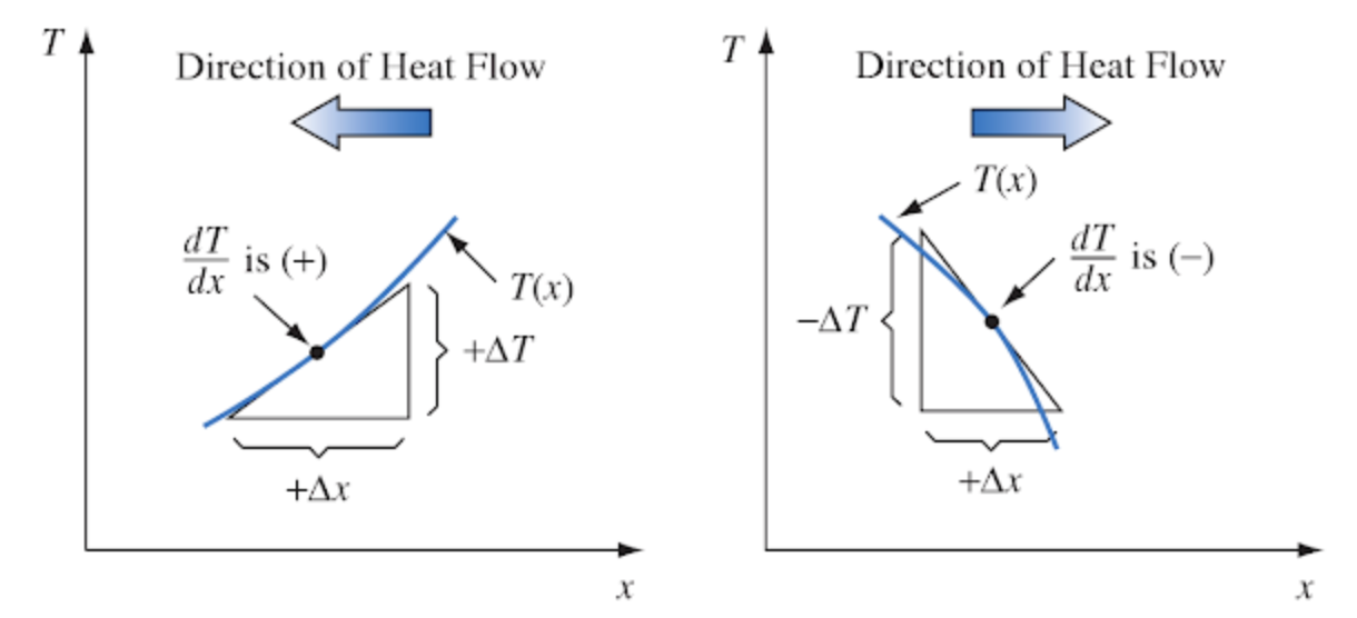
Figure 7.5: Sketch illustrating sign convention for conduction heat flow. From Kreith, F. 1973. P. 8.
The thermal conductivity depends on the molecular structure of the material. Some cooking pots have copper-coated bottoms because this metal transfers heat better than other materials. Home insulation materials reduce the flow of heat because they trap air which has a low thermal conductivity. The hollow centers of the hair shafts of some mammals reduces the conduction of heat along the fiber. The thermal conductivity can be calculated by measuring the heat flow when the temperature slope (Fig. 7.5) is one.
As an example of conduction, we will examine the heat flow between the alligator, Alligator mississippiensis, and substratum. We assume that the skin is the same temperature as the ground and that the animal is in good thermal contact with the surface (there are no air pockets reducing heat flow). The conduction exchange can now be calculated as follows. The thermal conductivity of fat is 0.20 \(W m^{-1} {^{\circ}C^{-1}}\) while the soil-rock range of conductivity is between 0.556 and 3.25 \(W m^{-1} {^{\circ}C^{-1}}\). Since the fat layer of 0.7 cm has a lower conductivity, it controls the rate of heat flow. Here we also assume that 0.5 \(m^2\) of the alligator at \(T_b = 22^{\circ}C\) are in contact with the ground at \(T_g = 30 ^{\circ}C\). In steady state, the conductive heat flux is then a linear function of the potential, as given in equation (7.7).
\[\begin{equation} Q_{cond} = \frac{k A_c}{x} (T_b - T_g) = \frac{0.198 \times 0.5}{0.007} (22-30) = -114 W \tag{7.8} \end{equation}\]
where- \(Q_{cond}\) is conduction (\(W\), negative since energy is flowing from the ground to the animal),
- \(T_b\) is body temperature of the alligator (\(^{\circ}C\)),
- \(k\) is the thermal conductivity of fat (\(W m^{-1} {^{\circ}C^{-1}}\)),
- \(T_g\) is ground temperature (\(^{\circ}C\)), and
- \(\Delta x\) is thickness of layer (\(m\)).
The TrenchR package includes similar functions for modelling convection based on whether the thermal conductivity of the animal or the substrate is the limited step. When animal conductance is the rate limiting step, \(Q_{cond}\) can be estimated as follows: \[Q_{cond}= A\cdot proportion\cdot k(T_g-T_b)/d, \] where \(k\) is thermal conductivity (\(W K^{-1} m^{-1} {^{\circ}C^{-1}}\)), \(T_g\) is ground (surface) temperature (K), \(T_b\) is body temperature (K), and \(d\) is the mean thickness of the animal skin (surface, \(m\)). This formulation assumes the organism has a well mixed interior rather than an interior temperature gradient.
When substrate thermal conductivity is the rate limiting step, \(Q_{cond}\) can be estimated as follows: \[Q_{cond}= A\cdot proportion \cdot(2K_g/D)(T_b-T_g),\] where \(K_g\) is the thermal conductivity of substrate (\(W K^{-1} m^{-1}\)) and \(D\) is the characteristic dimension of the animal (\(m\)).
The functions are available in R:
## [1] 1000## [1] 1.2Before proceeding to a discussion of convection, it is important to talk about an alternative view of conduction. It is possible to rewrite equation (7.8) as
\[\begin{equation} G = k_g (T_b - T_g) \tag{7.9} \end{equation}\]
The rate of heat flow is then equal to a conductance \(k_g\) times a potential, the temperature difference. The conductivity, area of contact and length have all been subsumed into \(k_g\). When working heat transfer problems, it is also common to speak and think of resistances to heat transfer. A resistance is simply the reciprocal of the conductance. If there is a large resistance to heat flow, there is a low conductance. Monteith (1973) and Campbell (1977) have adopted the resistance approach for describing mass and momentum fluxes as well as heat transport. This concept originated with Ohm’s Law where the electrical current flow is equal to the potential or voltage drop divided by the resistance of the material. Thus, the correspondence of a flux driven by a potential is called Ohm’s Law analogy. Kreith (1973, chapters 1 and 2) shows how radiation, convection and evaporation can also be thought of in these terms. It should be remembered though that in general the Ohm’s Law analogy, due to the complications introduced by turbulent mass and turbulent energy transfer, is an approximation (see Tennekes and Lumley 1973).
Conduction is often ignored in the heat transfer of plants and animals because one must know or make assumptions about the temperatures, boundary layer thickness, thermal conductivity, and contact resistance. There are not many actual measurements reported in the ecological literature but Mount (1968), Derby and Gates (1966), Gatesby (1977), and Thockelson and Maxwell (1974) offer some interesting examples of the importance of conduction.
7.3.3 Convection
Convection is the transfer of heat between solids and fluids (i.e., gases and liquids) or when fluids of different temperatures are in contact. Conduction takes place with nearby particles on the molecular level but the additional factor of the circulation of the fluid distinguishes convection from conduction. When there is no motion in the fluid except that caused by density gradients and by the resultant buoyant forces, this process is called “free convection.” If the fluid is moving relative to the other fluid or solid, the process is called “forced convection.” If the flow is turbulent, besides the molecular processes, there will be increased heat transfer caused by the bulk transport of fluid. Also, at certain fluid velocities, free and forced convection may both contribute to the convection term. Indeed convection is comprised of several complex physical processes occurring simultaneously.
Water and air are the two fluids that commonly interest the thermobiologist. Most aquatic organisms are at ambient water temperature; hence, convective transfer is unimportant because there is no temperature difference. Marine mammals, birds, a few large fish and turtles, however, maintain body temperatures above water temperature, which requires thick insulation (Bartholomew 1977, Schmidt Nielsen 1975). This is because the high specific heat (\(4.18 \times 10^3 J kg^-1 {^{\circ}C^{-1}}\)) and thermal conductivity (\(59.8 W m^{-2} {^{\circ}C^{-1}}\)) of water create a large heat loss. The extra heat transferred due to the movement of the fluid has not been examined for many organisms (but see Eskine and Spotila 1977 and Lueke et al. 1976). Although the specific heat and thermal conductivity of air are much less than for water, convection is still a significant mode of heat transfer for terrestrial organisms.
As with conduction, convective heat flow can be thought of as a potential (the difference in temperature between the surface of the object and the surrounding fluid) times a conductance. The conductance is most commonly written as the product of two terms as in equation (7.10):
\[\begin{equation} Q_{conv} = h_c A_c (T_s - T) \tag{7.10} \end{equation}\]
where- \(Q_{conv}\) is the convective heat flux (\(W\)),
- \(h_c\) is the convective heat transfer coefficient. (\(W m^{-2} {^{\circ}C^{-1}}\)),
- \(A_c\) is the area at object in contact with the fluid (\(m^2\)),
- \(T_s\) is the surface temperature of the object (\(^{\circ}C\)), and
- \(T\) is the fluid temperature (\(^{\circ}C\)).
Usually, \(A_c\), \(T_s\) and \(T\) can be evaluated. The heat transfer coefficient, on the other hand, is often a difficult parameter to estimate in the natural environment because of turbulence (Kowalski and Mitchell 1976, and Noble 1975).
TrenchR offers the following function for modelling convection. The function accounts for the proportion of the surface area in contact with the substrate, \(proportion\), and an enhancement factor multiplier, \(e_f\), that can be incorporated to account for increases in heat exchange resulting from air turbulence in field conditions. Conduction can be estimated as follows: \[Q_{conv}= ef\cdot h_c(A\cdot proportion)(T_a-T_b).\]
The function is available in R:
## [1] 0.2731369Generally, the heat transfer coefficient is evaluated as follows:
\[\begin{equation} h_c = \frac{Nu \, k}{D} \tag{7.11} \end{equation}\] where- \(h_c\) is the heat transfer coefficient (\(W m^{-2} {^{\circ}C^{-1}}\)),
- \(Nu\) is the Nusselt number,
- \(k\) is the thermal conductivity of the fluid (\(W m^{-1} {^{\circ}C}\)), and
- \(D\) is the characteristic dimension of the system (\(m\)).
The heat transfer coefficient, \(h_c\), is a value which has been averaged over the entire surface area of the system. The characteristic dimension \(D\) must be defined for each different geometric shape one wishes to consider. Commonly, one might use the diameter of a sphere or the widest point of a leaf in the direction of the wind. The Nusselt number is a non-dimensional number used to scale laboratory results to other wind velocity and fluid properties. Kreith (1973, page 317) gives two physical interpretations for the Nusselt number. It may be thought of ‘as the ratio of the temperature gradient in the fluid immediately in contact with the surface to a reference temperature gradient \((T_s - T)/D\)’ or the ‘ratio \(D/x\) where \(x\) is the fluid thickness of a hypothetical layer which, if completely stagnant, offers the same thermal resistance to the flow of heat as the actual boundary layer.’
In practice, another non-dimensional number, the Reynolds number, \(Re\), which is the ratio of inertial (\(\rho v^2\)) to viscous forces (\(\mu V/D\)), is introduced to account for the scaling effects of fluid velocity, geometry, and fluid properties (see Kreith 1973 or Cowan 1977 for a discussion of \(Re\)).
\[\begin{equation} Re = \frac{\rho vD}{\mu} \tag{7.12} \end{equation}\] where- \(\rho\) is the fluid density (\(kg\,m^{-3}\)),
- \(V\) is the fluid velocity (\(m s^{-1}\)),
- \(D\) is the characteristic dimension (\(m\)), and
- \(\mu\) is the fluid viscosity (\(kg m^{-1} s^{-1}\)).
For a particular geometry, a functional relationship between the Nusselt number and the Reynolds number can then be calculated from laboratory measurements (\(h_c\) versus \(V\)). Usually, the result is expressed as:
\[\begin{equation} Nu = a {Re}^b \tag{7.13} \end{equation}\] where \(a\) and \(b\) are determined by regression. The parameters will be different for different shaped objects (Kreith 1973). Then, using equation (7.12), the \(Nu\) can be calculated which in turn will yield the convection coefficient from equation (7.11). This procedure is the standard method used in engineering. In ecological studies, where one is concerned about the effects of wind speed and size and the geometry of the system is constant, the convection coefficient is sometimes given without specifically indicating the coefficient of equation (7.13) as in the following example. This approach is more direct and is fine to use as long as the student realizes what has been implied.
The Nusselt and Reynolds numbers and additional dimensionless groups are available in TrenchR as follows:
## [1] 0.4## [1] 0.0008333333TrenchR offers methods to estimate the convective heat transfer coefficient entails based on either empirical measurements (heat_transfer_coefficient()) or approximating the animal shape as a sphere (heat_transfer_coefficient_approximation()), which enables simplification while also producing an reasonable approximation [Mitchell 1976]. The functions approximate forced convective heat transfer as a function of windspeed \(V (m/s)\), the characteristic dimension \(D (m)\), the thermal conductivity of the air \(k (W m^{-1} K^{-1})\), the kinematic viscosity of the air \(nu (m^2 s^{-1})\), and the taxa or a generic shape. An additional, simplified function (heat_transfer_coefficient_simple()) provides a reasonable approximation based on \(V\) and \(D\) for most environmental conditions.
## [1] 9.936011heat_transfer_coefficient_approximation(V=3, D=0.05,
K= 25.7 * 10^(-3), nu= 15.3 * 10^(-6), "sphere")## [1] 43.37924## [1] 14.80412- \(Q_{conv}\) is the convective heat flux (\(W m^{-2}\), positive for heat flow from the leaf to the air),
- \(k_1\) is 9.14 (\(J m^{-2} {^{\circ}C^{-1}} s^{-1/2}\)),
- \(V\) is wind velocity (\(m s^{-1}\)),
- \(D\) is the characteristic dimension (widest point) of the leaf in the direction of the wind (\(m\)),
- \(T_s\) is the surface temperature of the leaf (\(^{\circ}C\)), and
- \(T_a\) is the air temperature (\(^{\circ}C\)).
After using this convection term \(Q_{conv}\) in the energy budget equation, Tibbals et al. (1964, page 538) concluded for similar energy environments “that . . . that the broad deciduous type leaf would be considerably warmer than the conifers . . .” and " . . . that the demand on transpiration is probably greatest per unit surface area for the broad-leaf plant than the conifers." (Also see Gates 1977.)
The theory of convective transfer is more complex than presented here. Although some additional material will be included in the problems, the reader may wish to refer to Kreith (1973), Monteith (1973) or Campbell (1977).
7.3.4 Evaporation
Evaporation is the process of water changing from a liquid to a gas. For animals, water can be lost through respiration, through special glands, or through any part of the skin. Water loss is usually a small component of the heat balance for animals but may be large for animals with moist skins. It usually increases quickly at higher temperatures. Figure 7.6 from Dawson and Templeton (1963), shows this effect for the collared lizard, Crotaphytus collaris. In general, the water loss, \(E\), is given by equation (7.15). Again, this is in the form of a potential divided by a resistance (an Ohm’s Law analogy). \[\begin{equation} E = \frac{C_o - C_a}{r_e} \tag{7.15} \end{equation}\] where- \(E\) is water loss (\(kg\,s^{-1}\)),
- \(C_o - C_a\) is the water vapor concentration difference between the surface (\(o\)) and the free atmosphere (\(a\)) (\(kg\,m^{-1}\)),
- \(r_e\) is the resistance to water vapor loss (\(s\,m^{-1}\)).
The TrenchR package incorporates a function based on empirically estimated relationships (Qevaporation) to estimate evaporation.
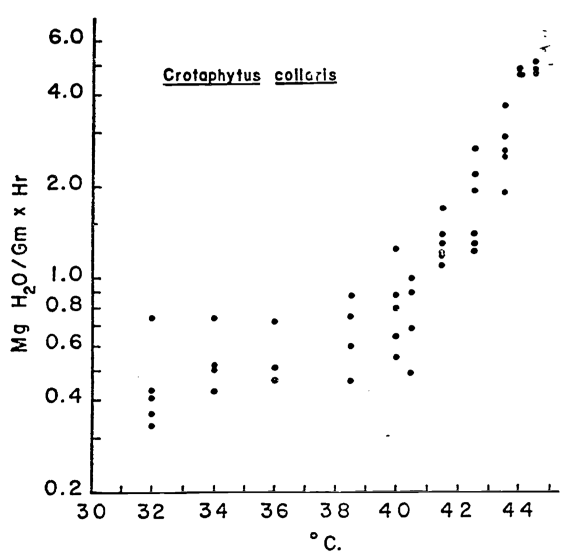
Figure 7.6: Relation of evaporative water loss to ambient temperature in collared lizards weighing 25-35g. Data represent minimal values at various temperatures for animals studied. (From Dawson, W.R., and J.R. Templeton. 1963. P. 231.)
The water vapor concentration at the surface of the water loss site may be saturated such as that of a leaf or a lung of a bird but it may be less than saturated as in the skin of a lizard. The concentration in the air is equal to the saturated concentration (at air temperature \(T_a\)) times the relative humidity. The resistance to water loss in the skin of a lizard will be controlled by the resistance to water movement in the skin and the boundary layer resistance. In a leaf, the total resistance to water loss is a combination of the stomatal resistance and the boundary layer resistance. But the water loss resistance from the moist skin of a frog was assumed to be equal to the boundary layer resistance only (Tracy 1976). In general, the boundary layer resistance is a function of the diffusion coefficient of water vapor in air and the boundary layer thickness. This thickness in turn depends on the size of the object as well as the wind speed.
To relate the water transport calculated in equation (7.15) to the energy balance, the mass flux \(E\) must be multiplied by the latent heat of evaporation \(L\). \(L\) can be closely approximated as a function of temperature. \[\begin{equation} L(T) = 2.50 \times 10^6 - 2.38 \times 10^3 T \tag{7.16} \end{equation}\] where- \(L(T)\) is the latent heat of evaporation (J kg-1),
- \(T\) is the surface temperature at the site of evaporation (°C).
As an example of the energy flux, the water loss at \(T_a = 40^{\circ}C\) for C. collaris is 0.8 mg of \(H_2 O\,g^{-1} {hr}^{-1}\) Correcting the units to kg \(s^{-1}\) for a 30 g lizard yields \(6.67 \times 10^{-9} kg\:s^{-1}\). Therefore, using equation (7.16), the energy loss for the animal is \(1.6 \times 10^{-2} W\). In this example, we have not calculated \(E\) explicitly, mechanistically accounting for wind speed or water vapor concentration of the environment, but animal physiologists often report evaporation as a function of air or body temperature only. These factors become more important when water loss is a larger fraction of the total energy budget or when one is concerned with the water balance of the organism (Welsh and Tracy 1977). Later in the text, a functional relationship to include these factors is given for water loss from a leaf. Generally, transpiration is a significant energy loss for plants which has led Monteith (1973) to make the distinction between “wet” and “dry” systems.