2.3 Functions of One Variable

2.3.1 Rates of Change

The simplest graph of a dynamic relationship is a straight line. The equation for a straight line is

$$\begin{equation} y = mx+ b \tag{2.1} \end{equation}$$

where $y$ and $x$ are variables, $m$ and $b$ are constants. An example of this relation is the oxygen uptake by the lobster. The oxygen consumption $(y)$ depends on the oxygen concentration $(x)$ in the surrounding environment, so that $y$ is a function of $x$. A typical graph of this function shown in Figure 2.1.

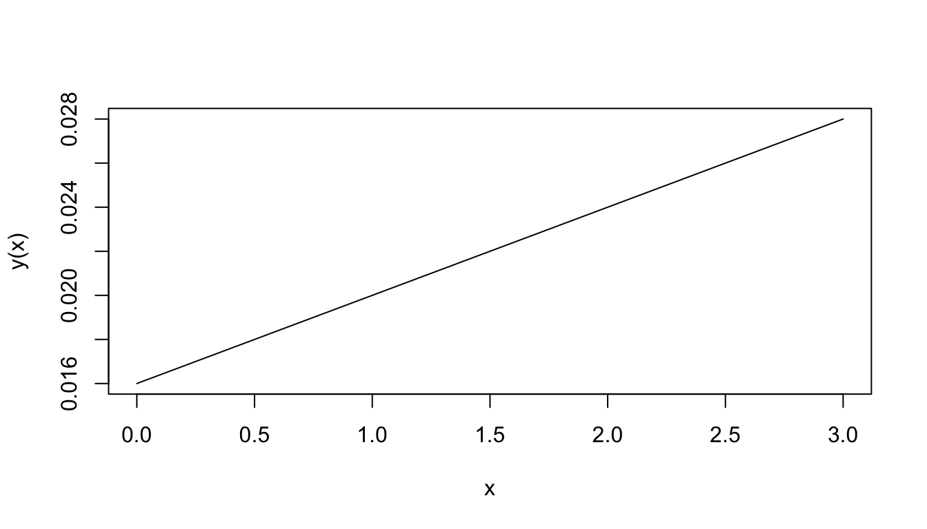
Figure 2.1: Oxygen consumption.

The equation for this function is $$y(x)=0.004x+0.016$$ The number 0.004 represents the slope of the line; that is, the ratio of the change in $y$ to the change in $x$. When $x$ changes by 1 unit, $y$ changes by 0.004 units. In this particular application, when the water O₂ concentration increases by one ml/l, the lobster O₂ consumption increases by 0.004 ml per hour-gm body weight. The slope ($m$ in Equation (2.1)) then represents the rate of change of $y$ with $x$.

When the graph is not a straight line, the function it represents is more complex than above and the rate of change cannot be expressed so easily. Note that for each unit change in $x$ in Fig. 2.1, $y$ changes by 0.004, regardless of the value of $x$. The rate of change is then constant. In the graph of Fig. 2.2, the rate of change is not constant. To see this, approximate Fig. 2.2 by two connected tangent lines (Fig. 2.3a) and note that the slope differs with each line. As the approximation improves (Fig. 2.3b), it uses more lines and thus presents more slopes. Using an infinite number of lines, we would duplicate the curve (in Fig. 2.2) and have a slope that changes with each value of $x$. The slope then depends on $x$ and clearly is not constant. In fact, one definition of the slope of a curve at a point is the slope of the tangent line at that point.

Note that the slope is ambiguous at the points where two straight lines meet (Figure 2.3a). We say the slope is “undefined” at such “corner” points.

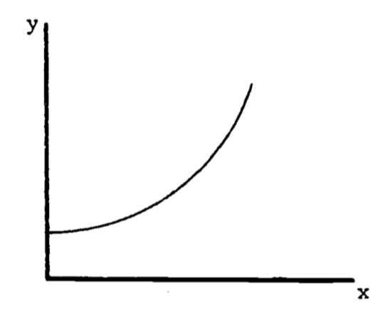
Figure 2.2: Example of a function with a changing slope.

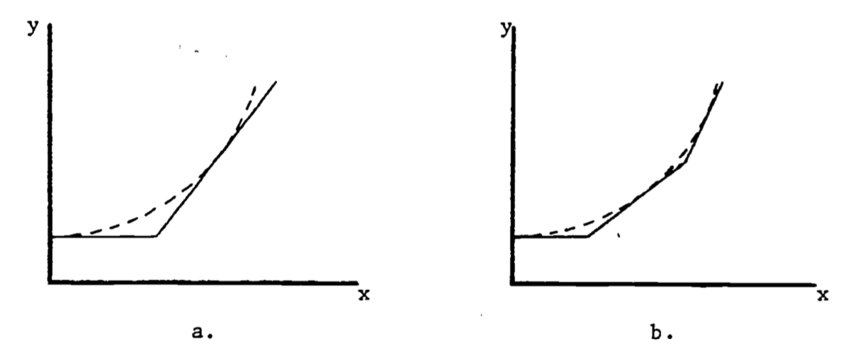
Figure 2.3: Approximations to the curve in Figure 2.

In general, the rate of change of a function is also a function of $x$ and possesses its own equation. The rate of change is denoted to $\frac{dy}{dx}$ reflect the ratio of the change in $y$ to the change in $x$. When the graph is a straight line, the equation for $y$ is $$y(x) = mx + b$$ and the rate of change is $$\frac{dy}{dx}=m$$ The rate of change is called the derivative. Its functional form depends on the equation for $y$. For example, an empirical relation between oxygen consumption $(Q)$ and body weight $(W)$ is $$Q=3W^2$$ The derivative of this function is $$\frac{dQ}{dW}=(3)(2W)=6W$$ The graph of $Q = 3W^2$ is given in Fig. 2.4a. The derivative at $W = 1$ represents the slope of the line tangent to the curve at the point where $W = 1$, as shown in Figure 4b. At $W = 1$, the slope is calculated to be $$\frac{dQ}{dW}=6(1)=6$$

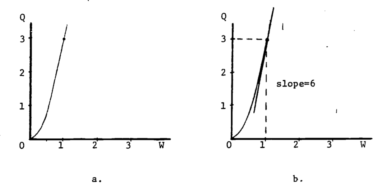
Figure 2.4: Derivative as the slope of the tangent line.

The number “$3$” in the formula $Q = 3W^2$, as well as the “$2$” in the exponent, are empirically determined and differ with body size and species. The general formula is $$\begin{equation} Q=aW^b \tag{2.2} \end{equation}$$ The derivative of this power function is $$\frac{dQ}{dW}=a\cdot b\cdot W^{b-1}$$ Table 2.1 gives the more common functions and their derivatives. For a more complete table, see any calculus text, or any math handbook (see Bibliography).

Table 2.1. Derivatives of Elementary Functions

$y(x)$	$dy/dx$
$x^n$	$nx^{n-1}$
$e^x$	$e^x$
$ln\:x$	$1/x$
sin $x$	cos $x$
cos $x$	-sin $x$

2.3.2 Composite Functions

When a function is composed of several simple functions its derivative can be evaluated in stages. In the simple cases where $y$ equals the sum or product of two functions, $f(x)$, $g(x)$, the rules for differentiation (finding the derivative) are: $$y(x)=f(x)+g(x),\;\;\;\;\frac{dy}{dx}=\frac{df}{dx}+\frac{dg}{dx}$$ $$y(x)=f(x)g(x),\;\;\;\;\frac{dy}{dx}=f(x)\frac{dg}{dx}+g(x)\frac{df}{dx}$$ For example, if $y(x)=x^2(x-1)+2x$, then $$\begin{align*} \frac{dy}{dx}&=x^2\frac{d(x-1)}{dx}+(x-1)\frac{d(x^2)}{dx}+2 \\ &= x^2(1)+(x-1)(2x)+2 \\ \end{align*}$$ When $y$ is a function of a function, the chain rule provides the differentiation method: $$\frac{dy}{dx}=\frac{dy}{du}\frac{du}{dx}$$ For the composite exponential function $y=e^{2x}$, we have $$u(x)=2x,\;\;\;\;y(u)=e^u$$ $$\frac{dy}{du}=e^u, \;\;\;\;\frac{du}{dx}=2$$ Therefore $$\frac{dy}{dx}=2e^u=2e^{2x}$$ The Gompertz growth curve is used occasionally to describe the population size $(N)$ of some species as a function of time $(t)$, and is given by the equation $$N(t)=ae^{-be^{-kt}}$$ where $a$, $b$, $k$ are constants. The derivative $dN/dt$ then represents the rate of growth of the population. Here the chain rule is applied twice: $$N(t)=ae^{u(t)},\;\;\;\;u(t)=-be^{-kt}$$ $$\frac{dN}{du}=ae^u$$ Write $u(t)$ as $u=-be^{v(t)}$ where $v=-kt$. Then $$\frac{dv}{dt}=-k,\;\;\;\;\frac{du}{dt}=\frac{du}{dv}\frac{dv}{dt}=-be^v(-k)$$ $$\frac{dN}{dt}=\frac{dN}{du}\frac{du}{dv}\frac{dv}{dt}=ae^u(-be^v)(-k)=abke^{-be^{-kt}}\cdot e^{-kt}$$

2.3.3 Higher Derivatives

The derivative $dy/dx$ of a function $y(x)$ is called the first derivative of $y(x)$. If we write $$\frac{dy}{dx}=g(x)$$ then differentiating $g(x)$ produces $$\frac{dg}{dx}=h(x)$$ which is called the second derivative of $y(x)$, and is written $\frac{d^2y}{dx^2}$.

Other notation used for the first derivative includes $y'$ and $\dot{y}$, for the second derivative, $y''$ and $\ddot{y}$. Since the second derivative is also a function, it too can be differentiated to give the third derivative, and so on. The $n^{th}$ derivative is written (there is no general dot notation) $$\frac{d^ny}{dx^n},\;\;\;\; y^{[n]}$$

2.3.4 Critical Points

The first and second derivatives can be used to determine three special points on the graph of the function, namely, the relative maxima, relative minima and the inflection points. The relative maximum is easily visualized: the curve rises, reaches a peak, and then falls. The peak is the relative maximum. It is relative because the curve may rise even higher in a different place on the graph. Similarly, the relative minimum constitutes a low point on the curve. An inflection point is best illustrated by an example.

The logistic growth function describing population size is $$N=N_0\frac{1+b}{a+be^{-kt}}=N_0(1+b)(1+be^{-kt})^{-1}$$ where $k$ is a growth coefficient, $N_o$ is the population size at $t=0$ and $N_0(1+b)$ represents the carrying capacity of the environment. The growth rate is then $$\begin{align*} \frac{dN}{dt}&=N_0(1+b)(-1)(1+be^{-kt})^{-2}(be^{-kt})(-k) \\ &=N_0(1+b)bke^{-kt}(1+be^{-kt})^{-2} \\ \end{align*}$$ The coefficient $k$ is always positive. In this example, we restrict $b$ to be greater than 1.

At a relative maximum, the tangent line is horizontal so the slope is zero. Then the maximum growth rate occurs when the derivative of the growth rate equals zero. $$\frac{d(dN/dt)}{dt}=0$$ or equivalently, $$\frac{d^2N}{dt^2}=0$$

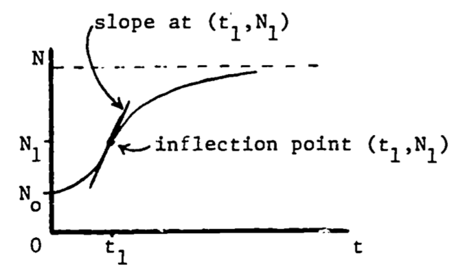
Figure 2.5: Maximum growth rate at the inflection point.

The second derivative of a function equals zero at the point of inflection, where the curvature changes from curving upward to curving downward, or vice versa. Then the maximum growth rate occurs when the population function $N(t)$ is at its inflection point (see Fig. 2.5). Since the slope is decreasing (leveling off) following the inflection point, and increasing before the inflection point, it is certainly maximal (steepest) at that point. This point can also be viewed as the relative maximum on the graph of the growth rate, $dN/dt$ (see Fig. 2.6).

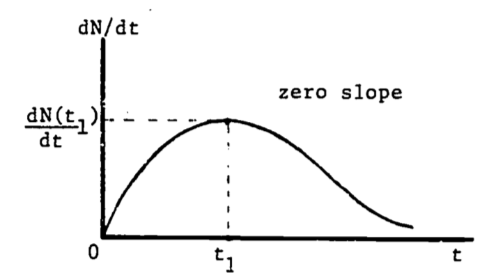
Figure 2.6: Growth rate as a function of time.

We now locate this point of maximum growth: $$0=\frac{d^2N}{dt^2}\;\;\;\;\;\mbox{at } (t_1, N_1)$$ $$0=\frac{d}{dt}[N_0(1+b)bke^{-kt}(1+be^{-kt})^{-2}]\;\;\;\;\mbox{at }(t_1, N_1)$$ $$0=N_0(1+b)bk^2e^{-kt_1}(be^{-kt_1}-1)(1+be^{-kt_1})^{-3}$$ Since all factors are positive except $(be^{-kt_1}-1)$, then $$0=be^{-kt_1}-1$$ Solving for $t_1$ gives $$t_1=(\frac{1}{k})ln\:b$$ and then substituting into the original expression for $N$, $$N_1=N_0(1+b)(1+be^{-k(\frac{1}{k}ln\,b)})^{-1}=N_0(1+b)/2$$ this says that the growth rate is highest when the population is one-half of the carrying capacity.