2.6 Problem Set

1. 1. The logistic population growth function satisfies the differential equation $$\frac{dx}{dt}=Ax(N-x)$$ where $x=x(t)$ is the population size and $N$ is the carrying capacity of the environment. Use this equation to show that the maximum growth rate (max $dx/dt$) occurs at the inflection point $x=N/2$. Assume $A$ is positive. (HINT: write the equation with $v = dx/dt$, and set $dv/dx = 0$).

  b. The “relative growth rate” is defined by $$R=\frac{1}{x}(\frac{dx}{dt})$$ where $dx/dt$ is as given in part (a). Let $x$ be given in “numbers of animals” and evaluate the units of $R$. The logistic curve is often used to describe “crowding effects” including intraspecies competition. Use the equation of part (a) to determine the value of $x$ which maximizes $R$, and explain this result in terms of crowding.

2. Leaves usually have small openings called stomata to allow passage of gases between their interior and exterior. Through them carbon dioxide passes in for capture by photosynthesis and the resulting oxygen passes out. Water vapor also escapes through the stomata, sometimes leading to dehydration. Thus plants have guard cells around the stomata to regulate their size. Action of the guard cells varies the shape of stomatal openings from a long narrow slit to nearly a circle. Throughout most of this variation the opening has approximately the shape of an ellipse with a constant length perimeter, typically about 35 $\mu$.
   A good approximation to the perimeter of an ellipse is $$P=2\pi\sqrt{(a^2+b^2)/2}$$ The area is given by $$A=\pi ab$$ Set $P=35$ and evaluate the area, $A$, in terms of just the width, $b$. Show that the area reaches a maximum when a=b, i.e., when the stomatal opening is a circle.

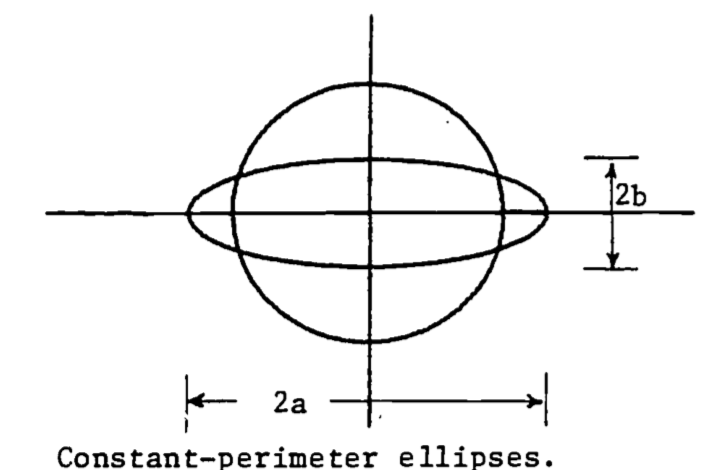
Figure 2.13: Constant-perimeter ellipses.

3. In the O₂ consumption model represented by equation (2.7), the variable $Q$ has units of $\mu$l/hr. Write $Q$ in ml/hr and find $\frac{\partial Q}{\partial m}$ for $W$ = 1000 mg. What are the units of $\frac{\partial Q}{\partial m}$? What might this derivative represent biologically? That is, why would a biologist be interested in this derivative?

4. A study of shape changes in nemerteans and flatworms (Alexander, 1968) theorizes that a basement membrane encloses the body and contains fibers which run in helices around the body. From Figure b, if the length $D$ of the fiber is fixed, then $l = D\cos\theta$ and when the shape is cylindrical, the circumference and volume are $2\pi r=D\sin\theta$, $v=\pi r^2l$.

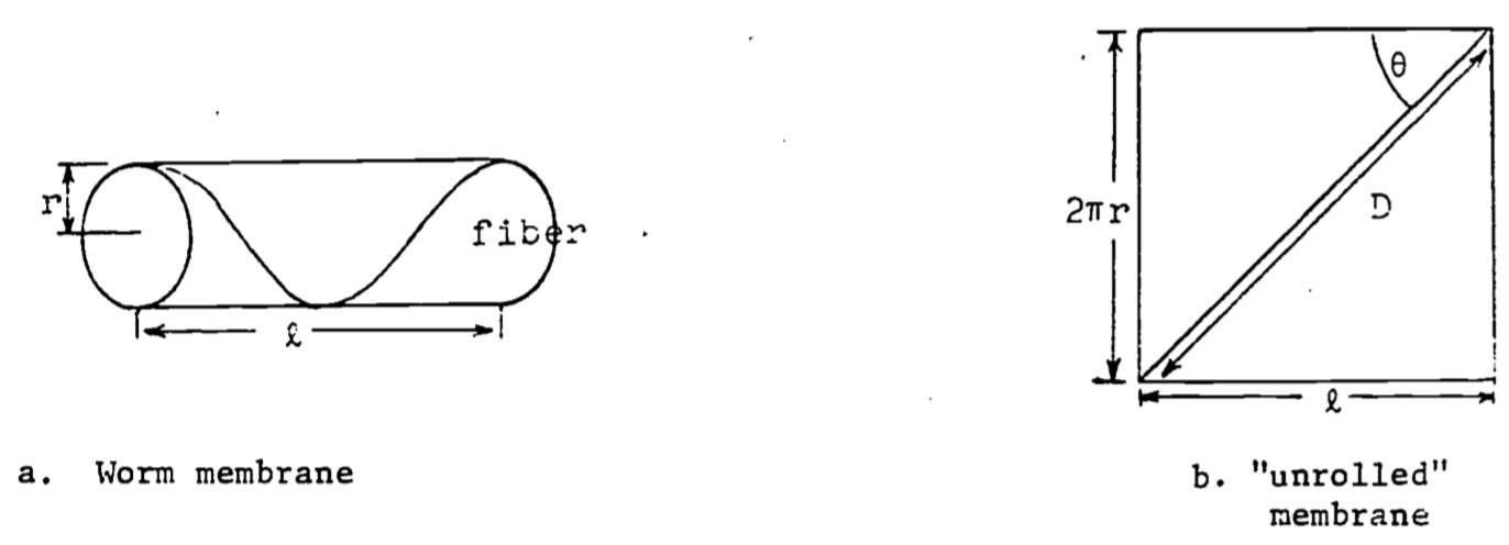
  a. Express $v$ as a function of $\theta$ (with $D$ a parameter) and show $v=0$ when $\theta=0$ or $\theta=\pi/2$ radians.

  b. Find $\theta$ which gives a maximum for $v$. Prove it is a relative maximum and not a relative minimum. Note that laboratory dissections show that in the relaxed worm the fibers run at about 55° to the axis of the body. Why would the relaxed worm have the maximum volume?

5. Studies of insect flight (Alexander, 1968) use the theory of “forced vibrations” to explain the muscle action responding to nervous stimuli. If the “forcing function” is assumed to be $$F\sin(2\pi nt),\;\;\;\;t=\mbox{time},\;\;\;\;F=\mbox{constant},$$ then the steady amplitude $A$ (magnitude of the vibrations) is given by $$A=F[(s-4\pi^2n^2m)^2+(2\pi nK)^2]^{-1/2}$$ where     $K$ = viscous damping coefficient
       $m$ = wing mass
       $n$ = frequency
       $s$ = stiffness of the vibrating medium
   Find the frequency $(n)$, called the resonant frequency, which gives the maximum amplitude.

6. This exercise verifies the location of the relative minimum in the example of “water falling across a rock face”. The function is $$z=x^3+y^3-3xy+15$$ Find all the critical points and determine which one is the relative minimum.

7. Heat transfer in soils depends on many factors; among them is the variation in the soil itself (de Vries, 1975).

Since most of the variation is in the vertical direction, a simple mathematical model is the one dimensional diffusion equation, $$C\frac{\partial T}{\partial t}=\frac{\partial}{\partial z}(\lambda\frac{\partial T}{\partial z})$$ where we define
    $T$ = temperature
    $t$ = time
    $z$ = vertical space coordinate
    $C$ = volumetric heat capacity
    $\lambda$ = thermal conductivity
When $C$ and $\lambda$ are uniform in depth and constant in time, we have the simple diffusion equation: $$\frac{\partial T}{\partial t}=a\frac{\partial^2 T}{\partial z^2}$$ where $a = \lambda/C$ is called the thermal diffusivity of the soil. The temperature at the surface gives boundary conditions for the model. For sinusoidal variation of surface temperature, we can write the boundary conditions as $$T(t,0)=T_a+\theta_0\cos\omega t$$ $$T(t,\infty)=T_a=\mbox{constant}$$ Show that the solution to this model is given by the following function: $$T(t,z)=T_a+\theta_0e^{-z/d}\cos(\omega t-z/d)$$ with $$d=(2a/\omega)^{1/2}$$ Be sure to verify that this function satisfies the diffusion equation and the boundary conditions.