15.7 Air Temperature
As with wind speed, there are two folders for air temperature, at different heights above the ground. In the case of air temperature, the height of the measurements in the weather station data used by New et al. (2002) was 120cm. And, as for wind speed, the microclimate model has been used to estimate values for 1cm above the ground.
Note also that, for the 1cm air temperatures, there are sub-folders specifying the substrate type and the shade level. This is because the estimated value of air temperature at this height is dependent on what shade and substrate type were used in the simulation. You have only been provided with two shade levels, 0 and 100%.
The next code chunk plots the air temperature at 120 cm for the two months at midday.
month<-1 # choose which month you want, 1 or 7 (i.e. Jan or Jun)
# read the file into memory
Tair120cm_jan<-brick(paste0(path,"air_temperature_degC_120cm/TA120cm_",month,".nc"))

month<-7 # choose which month you want, 1 or 7 (i.e. Jan or Jun)
# read the file into memory
Tair120cm_jul<-brick(paste0(path,"air_temperature_degC_120cm/TA120cm_",month,".nc"))

par(mfrow = c(1,2)) # set to plot 1 row of 2 panels
plot(Tair120cm_jan[[13]],main = "Tair 120cm, 12:00 January, deg C", zlim = c(0,40))
plot(Tair120cm_jul[[13]],main = "Tair 120cm, 12:00 July, deg C", zlim = c(0,40))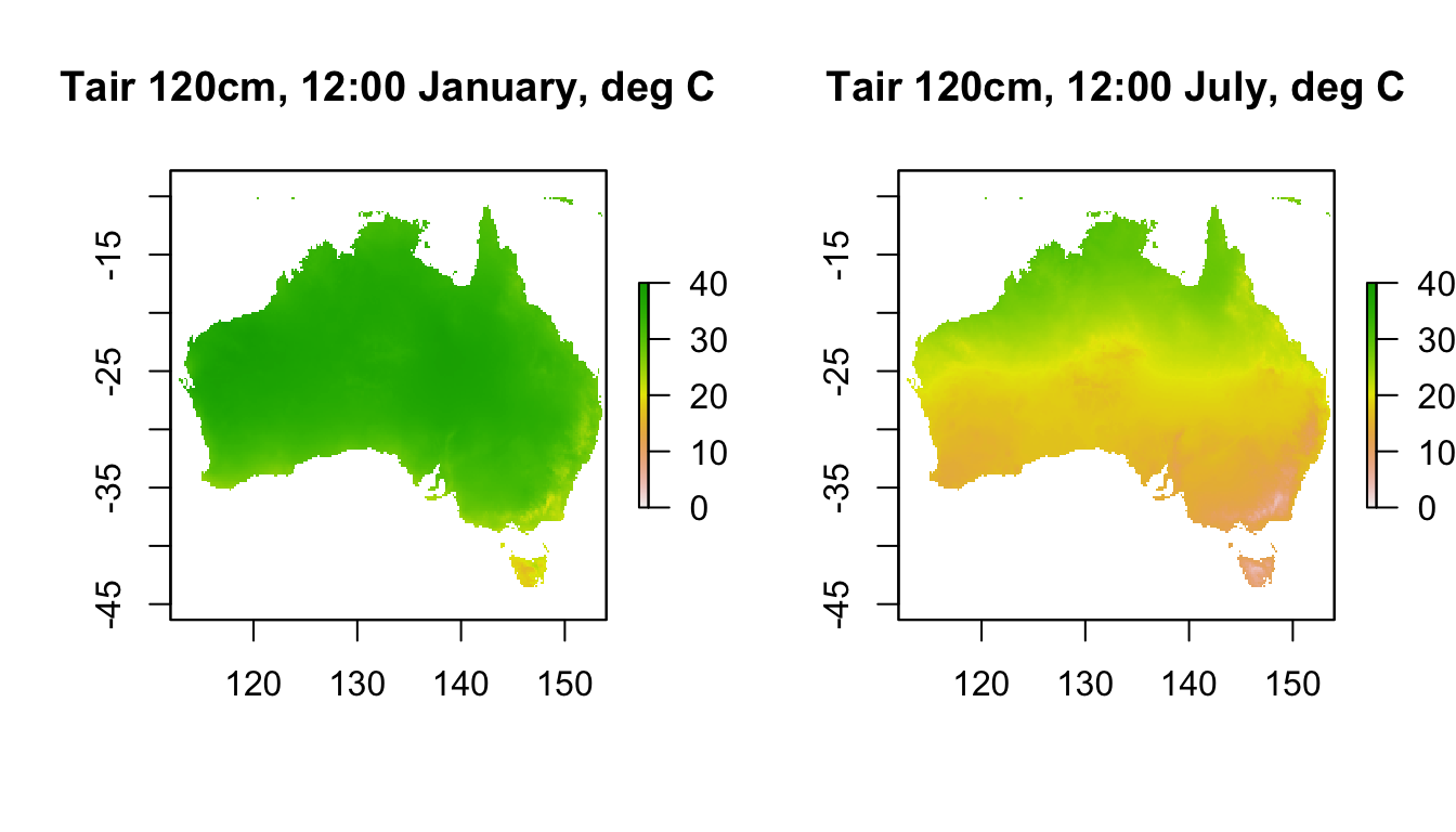
These weather station-height layers are what is typically used in correlative species distribution models.
Now we will plot the values at a 1cm height in 0% shade and in 100% shade.
month<-1 # choose which month you want, 1 or 7 (i.e. Jan or Jun)
shade <- 0 # choose which shade level you want, 0 or 100%
# read the file into memory
Tair1cm_0shade_jan<-brick(paste0(path,"air_temperature_degC_1cm/soil/",
                                 shade,"_shade/TA1cm_soil_",shade,"_",month,".nc"))

shade <- 100 # choose which shade level you want, 0 or 100%
# read the file into memory
Tair1cm_100shade_jan<-brick(paste0(path,"air_temperature_degC_1cm/soil/",
                                   shade,"_shade/TA1cm_soil_",shade,"_",month,".nc"))

month<-7 # choose which month you want, 1 or 7 (i.e. Jan or Jun)
shade <- 0 # choose which shade level you want, 0 or 100%
# read the file into memory
Tair1cm_0shade_jul<-brick(paste0(path,"air_temperature_degC_1cm/soil/",
                                 shade,"_shade/TA1cm_soil_",shade,"_",month,".nc"))

shade <- 100 # choose which month you want, 0 or 100%
# read the file into memory
Tair1cm_100shade_jul<-brick(paste0(path,"air_temperature_degC_1cm/soil/",
                                   shade,"_shade/TA1cm_soil_",shade,"_",month,".nc"))

par(mfrow = c(2,2)) # set to plot 2 rows of 2 panels
plot(Tair1cm_100shade_jan[[13]], main = "Tair 1cm 100% shade, 12:00 January, deg C", zlim = c(0,60))
plot(Tair1cm_100shade_jul[[13]], main = "Tair 1cm 100% shade, 12:00 July, deg C", zlim = c(0,60))
plot(Tair1cm_0shade_jan[[13]], main = "Tair 1cm 0% shade, 12:00 January, deg C", zlim = c(0,60))
plot(Tair1cm_0shade_jul[[13]], main = "Tair 1cm 0% shade, 12:00 July, deg C", zlim = c(0,60))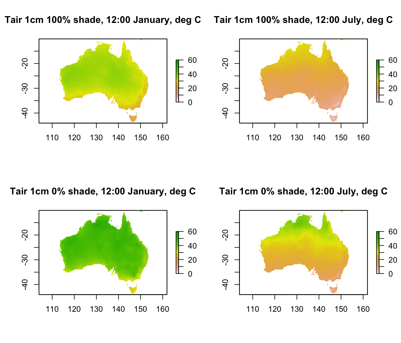
The values in 100% shade are almost identical to the 120cm values we plotted in the previous graph, and in this plot you can see that the values in 0% shade are much hotter than both the 100% shade 1cm and the 120cm air temperatures. Would this be the case at night? (take a look yourself to see the answer)
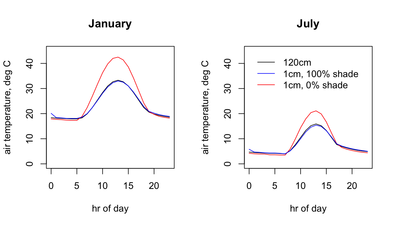
Next is some code to extract and plot the hourly values at the Flinders Ranges site for each month and height/shade level.
# extract data for all layers in 'Tair120cm_jan' at location 'lon.lat'
Tair120cm_jan.hr = t(extract(Tair120cm_jan, lon.lat))
# extract data for all layers in 'Tair120cm_jul' at location 'lon.lat'
Tair120cm_jul.hr = t(extract(Tair120cm_jul, lon.lat))
# extract data for all layers in 'Tair1cm_0shade_jan' at location 'lon.lat'
Tair1cm_0shade_jan.hr = t(extract(Tair1cm_0shade_jan, lon.lat))
# extract data for all layers in 'Tair1cm_0shade_jul' at location 'lon.lat'
Tair1cm_0shade_jul.hr = t(extract(Tair1cm_0shade_jul, lon.lat))
# extract data for all layers in 'Tair1cm_100shade_jan' at location 'lon.lat'
Tair1cm_100shade_jan.hr = t(extract(Tair1cm_100shade_jan, lon.lat))
# extract data for all layers in 'Tair1cm_100shade_jul' at location 'lon.lat'
Tair1cm_100shade_jul.hr = t(extract(Tair1cm_100shade_jul, lon.lat))

# plot air temperature at 120cm in January as a function of hour,
# as a line graph (using type = 'l'), in black
par(mfrow = c(1,2)) # set to plot 1 row of 2 panels
plot(Tair120cm_jan.hr ~ hrs, type = 'l', main = "January",
     ylab = "air temperature, deg C", xlab = "hr of day", col = 'black', ylim = c(0,45))
# plot air temperature at 1cm in 0% shade in January as a function of hour,
# as a line graph (using type = 'l'), in red.
points(Tair1cm_0shade_jan.hr ~ hrs, type = 'l', col = 'red')
# plot air temperature at 1cm in 100% shade January as a function of hour,
# as a line graph (using type = 'l'), in blue.
points(Tair1cm_100shade_jan.hr ~ hrs, type = 'l', col = 'blue')

# plot air temperature at 120cm in July as a function of hour,
# as a line graph (using type = 'l'), in black
plot(Tair120cm_jul.hr ~ hrs, type = 'l', main = "July",
     ylab = "air temperature, deg C", xlab = "hr of day", col = 'black', ylim = c(0,45))
# plot air temperature at 1cm in 0% shade in July as a function of hour,
# as a line graph (using type = 'l'), in red.
points(Tair1cm_0shade_jul.hr ~ hrs, type = 'l', col = 'red')
# plot air temperature at 1cm in 100% shade July as a function of hour,
# as a line graph (using type = 'l'), in blue.
points(Tair1cm_100shade_jul.hr ~ hrs, type = 'l', col = 'blue')

legend(0, 45, c("120cm", "1cm, 100% shade", "1cm, 0% shade"),
       col = c("black", "blue", "red"), lty=c(1, 1, 1), bty = "n")