16.5 Mapping the cold limits of the Desert Iguana

First, let’s work out the radiation required for the Desert Iguana to be 3 degrees C, the low body temperature threshold for survival. This is row one in our dataset.

a_max <- pars$abs_max[1] # get the maximum solar absorptivity value, choosing row 1
D <- pars$D[1] # diameter, m
T_b_lower <- pars$T_b[1] # body temperature, deg C
M <- pars$M[1] # metabolic rate, W/m2
E_ex <- pars$E_ex[1] # evaporative heat loss from respiration, W/m2
E_sw <- pars$E_sw[1] # evaporative heat loss from sweating, W/m2
k_b <- pars$k_b[1] # thermal conductivity of the skin, W/(m C)
K_b <- k_b/pars$d_b[1] # thermal conductance of the skin, W/(m2 C)
epsilon <- 1 # emissivity

Now, let’s define our input arguments for wind speed and air temperature as the microclim grids for North America in January - the coldest month in this part of the world.

V <- wind_jan_NAm # wind speed, m/s
T_air<-Tair_jan_NAm # air temperature range to consider, degrees C

Finally, we can run the Qabs_ecto function.

# compute the total radiation load for each air temperature and wind speed combination that would 
# give a Tb of 3 degrees, the lower survivable limit
Q_abs_lower <- Qabs_ecto(D = D, T_b = T_b_lower, M = M, E_ex = E_ex, E_sw = E_sw, K_b = K_b, epsilon = epsilon, T_air = T_air, V = V)

Now we have the amount of radiation needed at each air temperature and wind speed combination available across North America through each hour of the day such that a Desert Iguana in the open would be 3 degrees C. Let’s plot that for 4am and 12pm.

par(mfrow = c(1,1)) # set to plot 1 row of 2 panels
plot(Q_abs_lower[[5]], main = "radiation required (W/m2), 4am January", zlim = c(-1000, 1300))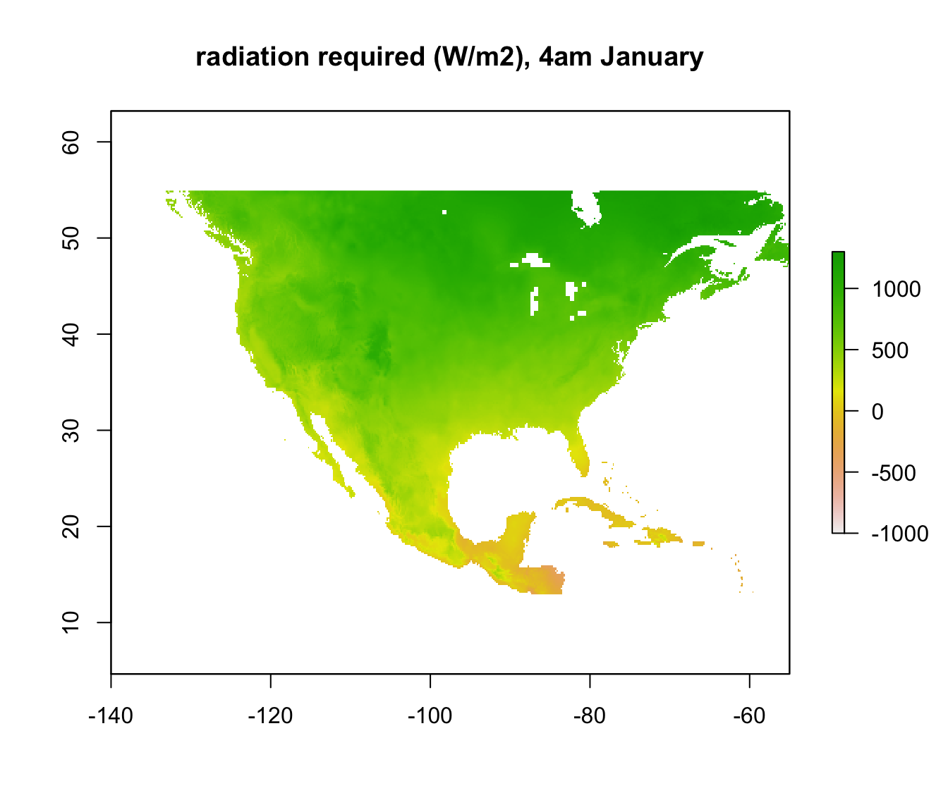

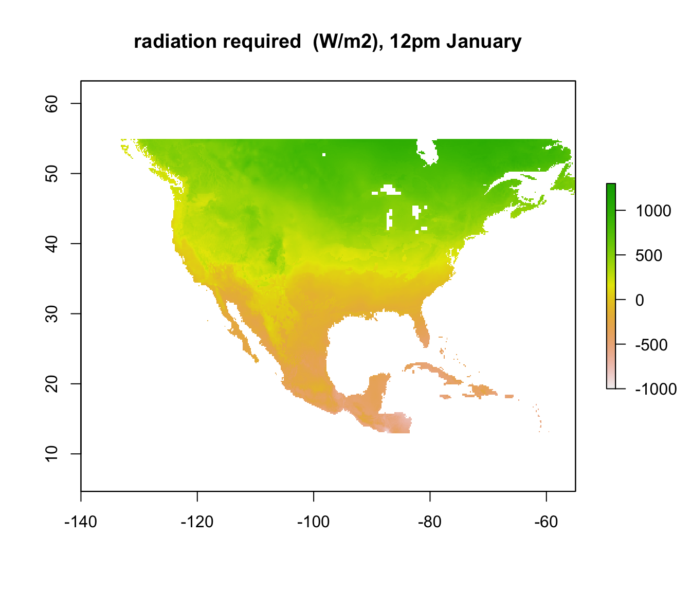
plot(Q_abs_lower[[13]], main = "radiation required  (W/m2), 12pm January", zlim = c(-1000, 1300))

Note that some areas are negative! You can’t have negative radiation - in such places, it would clearly be physically impossible to be colder than 3 degrees C due to the particular combination of wind speed and air temperature at that time and location. The air temperature is simply too high, no matter what the ground or sky temperature is. Those places are thus within the climate space of the Desert Iguana in terms of cold tolerance.

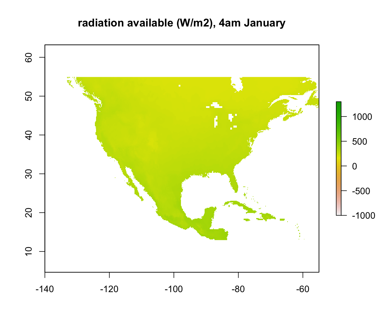
In other places, however, where the required radiation is positive, there still may not be enough radiation available to be 3 degrees C. We want to know where those places are. We have already calculated the available radiation at each place and time - the ‘Q_rad_Jan_NAm’ and ‘Q_rad_Jan_NAm’ grids which should still be in R’s memory. Let’s replot the ones for January at 4am and 12pm again for comparison.

plot(Q_rad_jan_NAm[[5]], main = "radiation available (W/m2), 4am January", zlim = c(-1000, 1300))

plot(Q_rad_jan_NAm[[13]], main = "radiation available (W/m2), 12pm January", zlim = c(-1000, 1300))

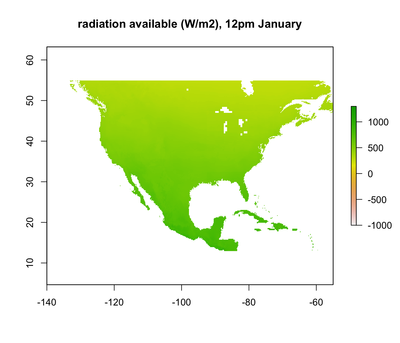
If we subtract the required radiation values from the available radiation values, all the places we get a positive result will be the places that are too cold to be 3 degrees C or warmer. The next code chunk makes this calculation and plots it, making the upper z-limit zero so only areas where the lizard would be 3 degrees C or warmer are coloured.

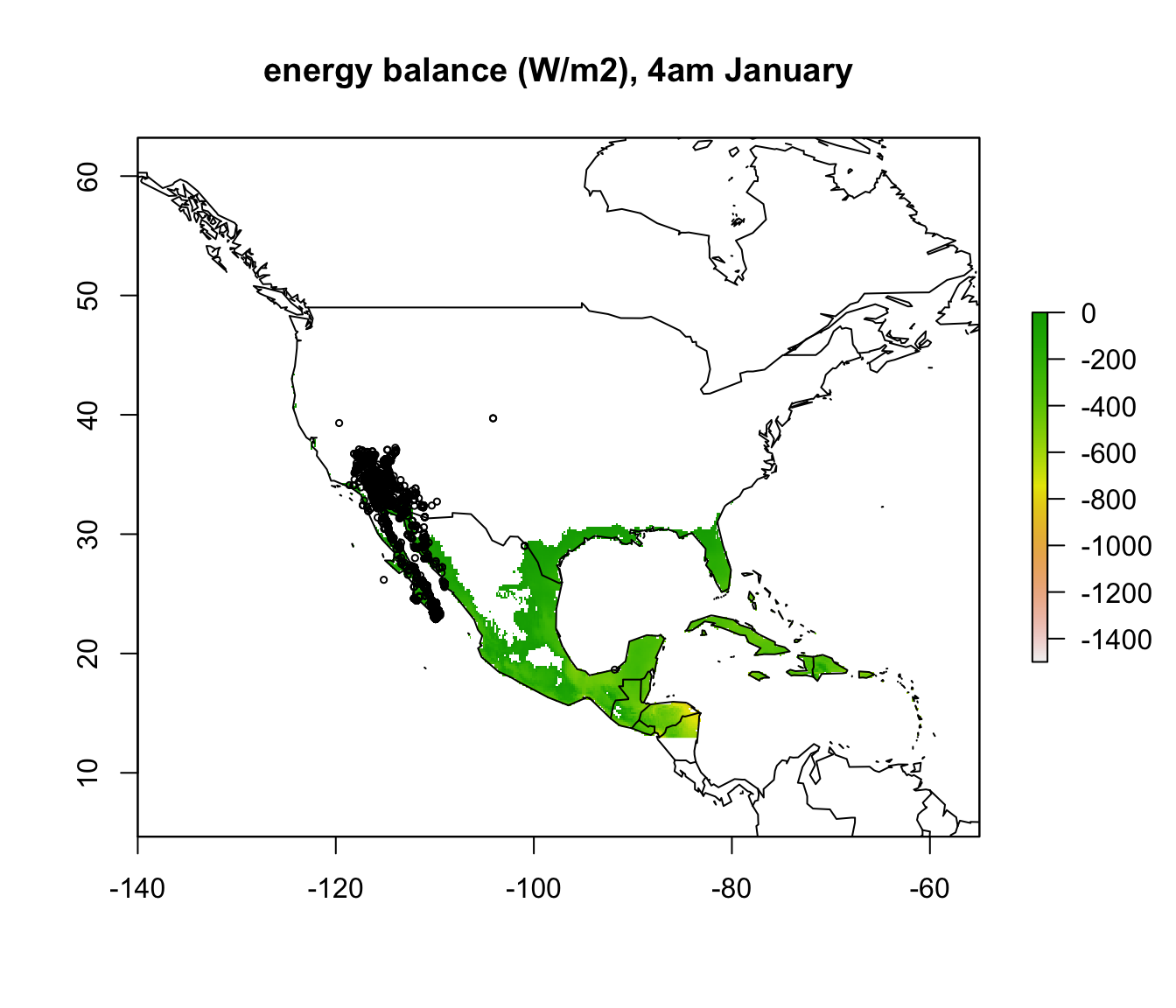
enbal_cold <- Q_abs_lower - Q_rad_jan_NAm # subtract required from available radiation for 3 degrees Tb
plot(enbal_cold[[5]], main = "energy balance (W/m2), 4am January", zlim = c(-1500,0))

plot(enbal_cold[[13]], main = "energy balance (W/m2), 12pm January", zlim = c(-1500,0))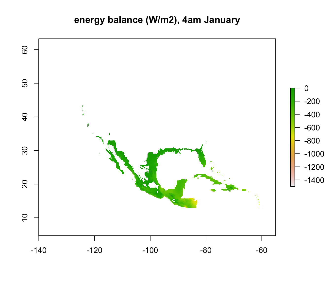

To make things a bit clearer, you can add outline map of the world using the following code.

library(maps)
map('world', add = TRUE)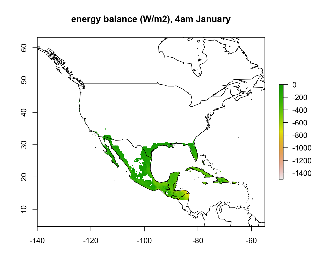

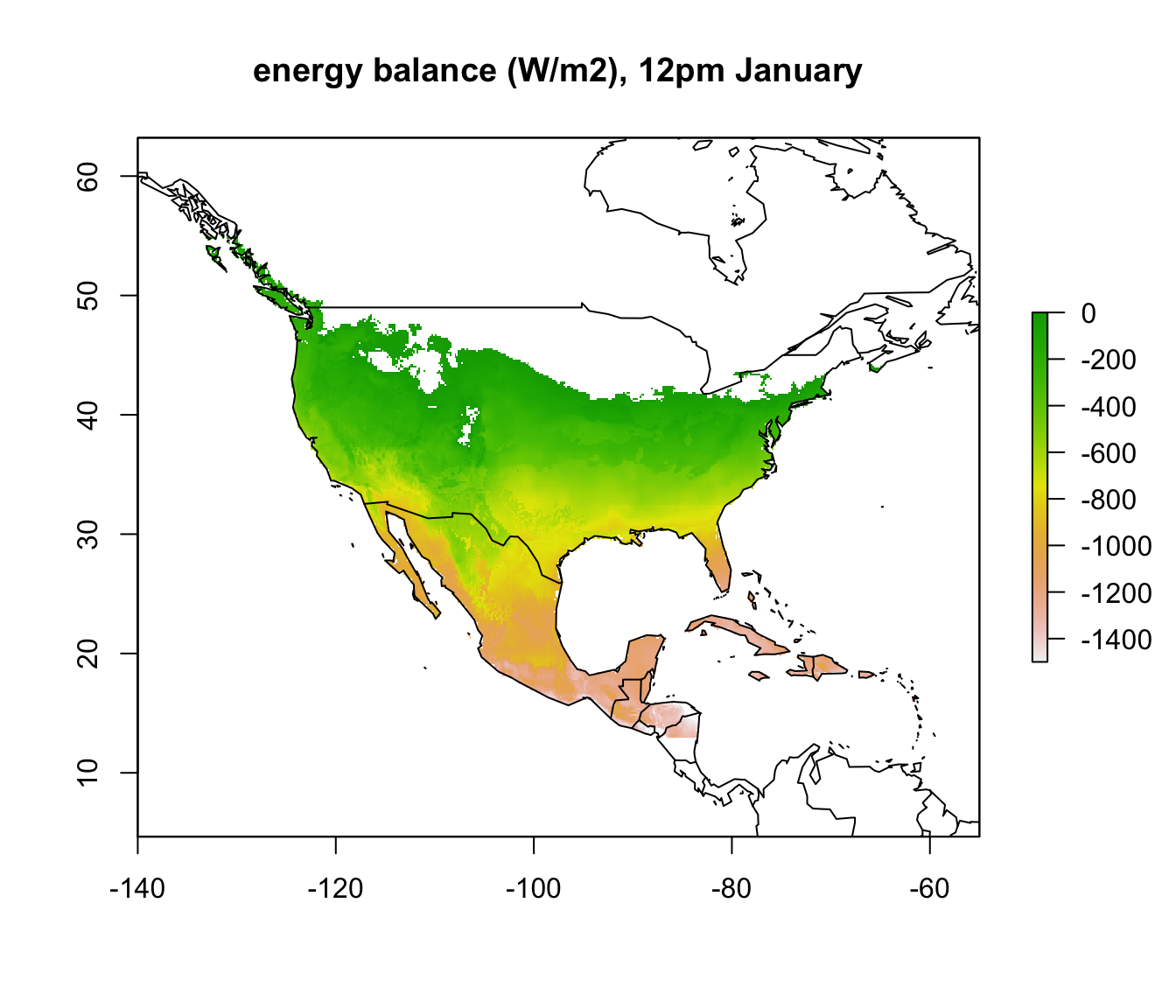
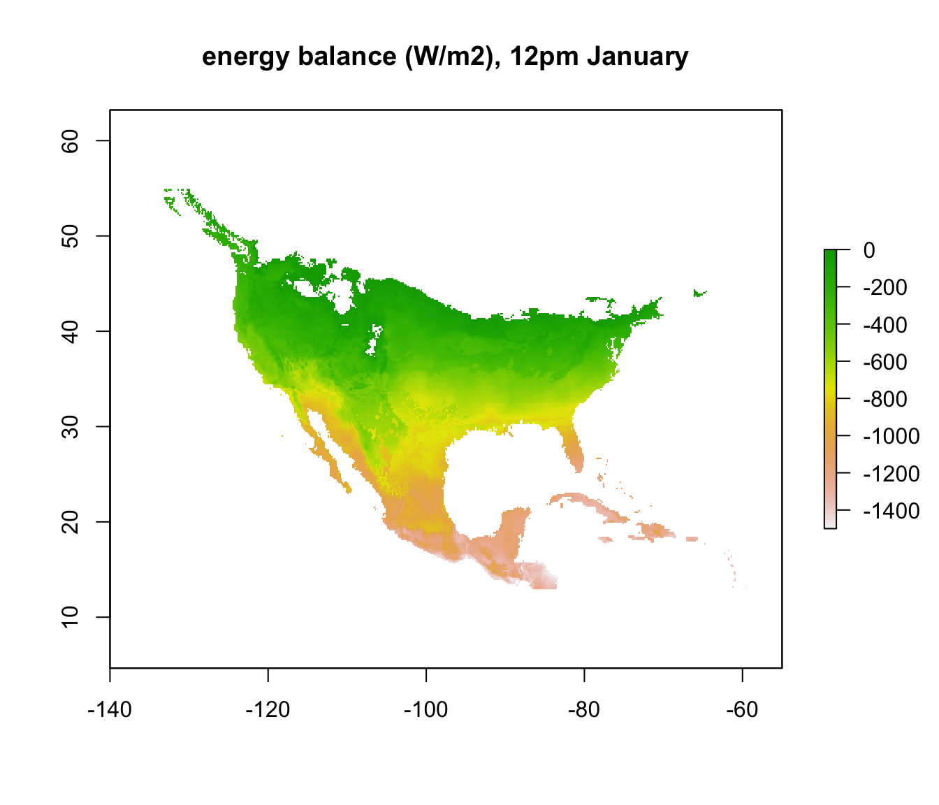
In parts of Mexico and Central America you can see that it is warm enough for a Desert Iguana to be sitting out in the open at 4am in January and be warmer than 3 degrees, and the area where this is the case is much greater at midday. Let’s now plot the actual distribution of the Desert Iguana onto these maps. You’ve been supplied with this data in the file ‘dipso_dist.csv’ which was obtained using the gbif function of the ‘dismo’ package, specifically the code:

library(dismo)
dipso_dist <- gbif("Dipsosaurus", "dorsalis", geo = T)
write.csv(dipso_dist, file = "dipso_dist.csv")

You can read it in with dipso_dist<-read.csv("dipso_dist.csv") and add the points to each map with the following code inserted after each plot:

points(dipso_dist$lon, dipso_dist$lat, col = "black", cex = 0.5)

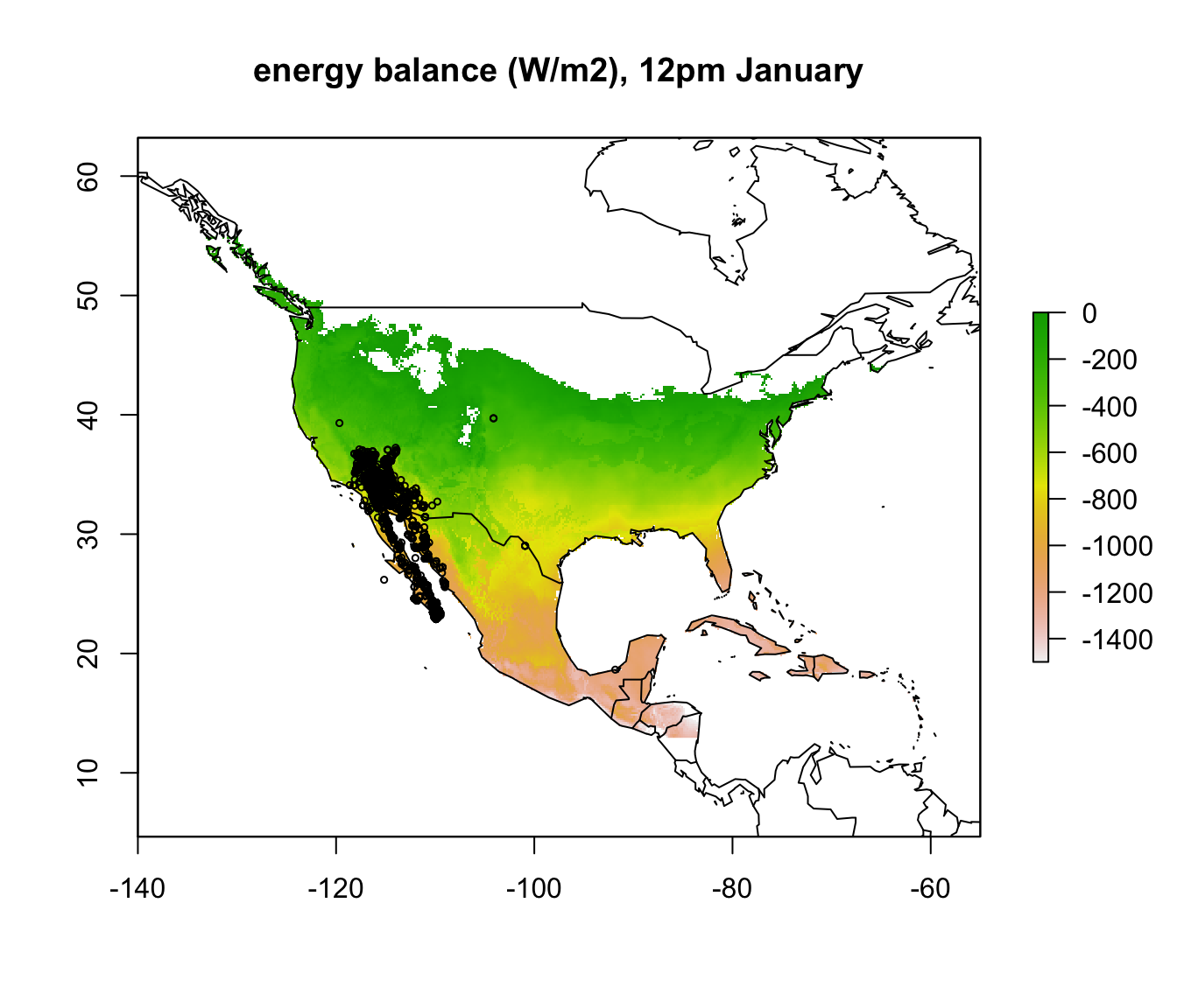
What would you conclude about cold as a limiting factor on the distribution of the Desert Iguana at this point?