2.8 Additional Problems
- In the example in the text treating oxygen consumption(see also problem 3 above), the oxygen consumption \((Q)\) depended on both the activity level \((m)\) and the dry weight \((W)\): \[Q=0.00187(m+1)W^{0.7}\] where the units of \(Q\) are mlO2/hr. For this exercise, we use the correspondence \[Q \rightarrow z,\;m \rightarrow x,\;W\rightarrow y\] so that the equation is \[z=0.00187(x+1)y^{0.7}\]
Evaluate the first partial derivative \(\partial z/\partial x\). If you plot \(\partial z/\partial x\) with increasing \(x\), is it supposed to be a straight line, concave upward, concave downward?
Now reverse the roles of \(x\), \(y\): evaluate \(\partial z/\partial y\).If you were to plot \(\partial z/\partial y\) against \(x\), is the shape supposed to be a straight line, circle, parabola … ?
This exercise illustrates how different parameter values can affect the properties of a function and its critical points. Function 2 is used in this exercise and is a simple polynomial in two independent variables: \[z=(P1)x^2+(P2)y^2\] Calculate all the partial derivatives needed to locate and classify a critical point. Set values for \(P1\), \(P2\) and evaluate the critical point.
When a beam of rectangular cross-section is cut lengthwise from a log, its strength can sometimes be well described by the following function: \[S=kWD^2\] where
\(S\) = strength of beam
\(W\) = width of beam
\(D\) = depth of beam
as shown in Figure 2.14, and where \(k\) is a constant which depends on the type of tree used. Assume that the log is circular in cross-section and that the beam is cut so each corner reaches the outside of the log, as shown. Assume \(k\) = 0.1. Find the width and depth of the beam which give the maximum strength. Assume the radius of the log is \(r\).
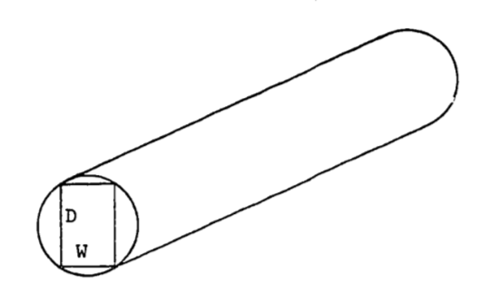
Figure 2.14: Rectangular beam cut from a log.
- Animal populations newly introduced into a region have been observed to increase rapidly in number and soon thereafter to fall drastically (Caughley 1970a, b) as indicated in Figure 2.15. One theory is that the population at first “senses” an infinite food supply and then reproduces rapidly to the point of overgrazing the area. The birth rate remains the same but the death rate (perhaps of young) dramatically increases until the population is low enough to match the food supply. The population then increases more slowly and seems to stabilize. Migration is also involved but is poorly understood. The second population rise to a “steady-state” suggests some adaptation or social “learning” by the population concerning their new environment.
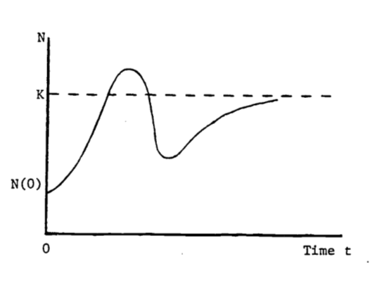
Figure 2.15: Population dynamics of introduced species.
Consider the logistic equation written as follows: \[N(t)=K(1+be^{-rt})^{-1}\] where \(K\), \(b\), \(r\) are positive constants, and \(N(0) < K\). In an attempt to describe the behavior in Figure B, one could modify the above logistic function by allowing \(r\) to vary over time, i.e. \(r = r(t)\). Can the population ever exceed \(K\)? If not, then this modified logistic function is not a good model. Answer this for a general \(r(t)\) in any fashion: by examining the function \(N(t)\) itself, by evaluating the maximum of \(N(t)\), etc.
An alternate model is developed if the discreteness of the population is taken into account. The logistic function in part (a) assumes that the population size, \(N(t)\), will change continuously as time changes. In certain species, populations do not change size smoothly (see Sladen and Bang 1969). The breeding time is a short period, once a year so that many off-spring are born at the same time. The population size then increases in large jumps. This discrete change is not modeled well by differential equations. A closely related field is the study of “difference equations” (see Goldberg 1958) where discrete changes are allowed. The derivative of the logistic function satisfies the differential equation \[\frac{dN(t)}{dt}=rN(t)\Big(\frac{K-N(t)}{K}\Big)\] From this formulation, we see that the logistic model assumes that the population is always aware of how far from the carrying capacity is the current population size and so continuously adjusts for this difference. (Note that the derivative depends on this difference, \(K-N(t)\)). Actually, plentiful food one season may cause too many births the following season, with a definite time lag between abundant food and severe overpopulation and with few adjustments in between.
The computer is used here to illustrate this inadequacy of differential calculus. The derivative above is replaced by a difference: \[\frac{N(t+1)-N(t)}{(t+1)-t}=rN(t)\Big(\frac{K-N(t)}{K}\Big)\] This model assumes the population changes only once per time period (e.g. annually) and is unable to adjust in between. Is this more or less realistic than the original logistic model? How would you include social or genetic “learning” into the model? That is, once the population size rises and then falls, what parameters might change in the model so that the next rise would be more gradual?
- The reaction \((Y)\) of the body to a dose \((X)\) of drug can be represented by the function: \[\begin{align*} Y(X)&=X^2(P1/2-P2\cdot X/3) \\ &=\frac{P1}{2}X^2-\frac{P2}{3}X^3 \\ \end{align*}\]
where \(P1\) and \(P2\) depend on certain body characteristics and on the maximum dosage which can be administered. \(Y\) indicates the strength of the reaction, measured in millimeters of mercury if blood pressure is being tested, or perhaps degrees Celsius if change in body temperature is being measured.
Find the dose that has “maximum sensitivity,” i.e. where the rate of increase of \(Y\) is greatest. Is this “critical point” a maximum or minimum for \(Y\)"? What is this point called on the graph for \(Y\)?