14.4 Origins of Turbulence
In the description of turbulence, it was noted that it is an ubiquitous property of almost all natural flows. It is of utmost importance in many processes due to its superior mixing and transport properties, while at the same time being very difficult to work with quantitatively due to its random nature. Two questions remain to be dealt with in this module: what is the origin of turbulence, and how can we quantify the transport which results without being overwhelmed by intractable complexities.
As discussed by Vennard and Street (1975) and Cowan (1979a), there are two flow regimes of interest in physical and biological processes: laminar and turbulent. Laminar flow is smooth, orderly and predictable, in contrast to turbulent flow. For a given flow geometry, one can predict by the value of the Reynolds number (\(Re\)) whether the flow is laminar, turbulent, or in a state of transition. The Reynolds number is a combined measure of fluid velocity, viscosity, density and a characteristic dimension. In essence, laminar flow becomes turbulent when small perturbations or instabilities in the flow are provided with a sufficient input of energy to grow and destroy the orderly nature of the laminar flow. In any given situation, one can think of an increase in the Reynolds number as a velocity increase, since the other parameters presumably would not change. A large Reynolds number corresponds to a large velocity and thus a large energy input. Therefore beyond some critical point, a large Reynolds number indicates that the flow instabilities will be able to grow and cause the flow to become fully turbulent. The flow geometry, including the roughness of any surfaces in contact with the flow, can have a dramatic effect on the values of the Reynolds number which define the transition zone between laminar and turbulent flow.
14.4.1 Viscosity and Laminar Shear Flows
As has been indicated, a source of energy is required to cause turbulent flow. Indeed, turbulence requires a continuous energy input, otherwise it rapidly decays due to frictional losses as a result of the viscosity of the fluid. Two sources of energy input exist to maintain turbulence in common flows. The first source is shear in the mean flow, where friction between the surface and the fluid causes energy from the mean flow to be diverted into the creation of turbulent velocity fluctuations. The second source derives from the heating of the fluid at the surface, which causes the fluid to rise generating turbulence. These mechanisms are known respectively as mechanical and thermal (convective, buoyance driven) turbulence. To gain some insight into these turbulence maintenance mechanisms, a fundamental understanding of viscosity and shear flows is essential, starting with laminar flow and progressing from there into the more complex turbulent flow case.
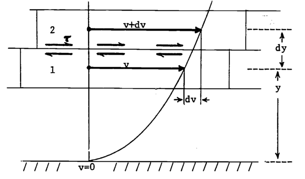
Figure 14.5: Laminar shear stress (T) between two regions, where velocity (v) depends on distance (y) from the bottom, after Vennard and Street (1975).
Consider the laminar flow of a fluid over a smooth horizontal surface as depicted in Fig. 14.5. Observations reveal that a velocity profile exists over the surface. In this case, from a condition of zero velocity right at the surface, the velocity increases with distance from the surface, indicating that there is relative motion between fluid layers. This is illustrated by consideration of the two infinitesimal fluid layers in Fig. 14.5. Two particles (1 and 2) in adjacent layers move distances of \(vdt\) and \((v+dv)dt\) in the time interval \(dt\). Thus we say that the fluid is sheared because the slope of a line connecting points 1 and 2 tends to increase with time. It should be evident then that a frictional force must exist between the fluid layers, otherwise the velocity profile would be uniform right down to the surface. This frictional force produces a shearing stress (\(\tau\)), and this stress has been found by observation to vary linearly with the velocity gradient (\(dv/dy\) in our example). The constant of proportionality in this relation is termed the viscosity coefficient (\(\mu\)), and we may write the relationship, known as Newton’s law of viscosity, as \[\tau = \mu \frac{dv}{dy}\] Viscosity is the result of molecular momentum exchange (a subject discussed subsequently in the discussion of mixing length theory) and cohesion between fluid layers, giving rise to the tangential shearing stress. Most fluids of interest here (e.g., air and water) obey the above relation, and are known as Newtonian fluids. (See e.g. Vennard and Street 1975, p.16 ff for a more detailed discussion.)
Although most flows in nature are turbulent, there are notable exceptions. For example, Cowan (1977b) treats the flow environment of plankton. Their movement can be closely approximated in many cases by treating the flow they encounter as laminar. (With their small diameter and sinking velocity, the Reynolds number here is quite small.) However, as is pointed out, the sea itself may be turbulent, as most flowing water certainly is (see Cowan 1979b or Ealgeson 1970), which may invalidate this simplified approach in some applications.
14.4.2 Turbulent Shear Flow
As has been described earlier (see also Tennekes and Lumley 1972 or Cowan 1977), turbulent flow is a random and irregular variation of velocity which can be thought of as being superimposed upon a steady mean flow velocity. The concept of an eddy was used to visualize that part of the flow responsible for this variation. It seems apparent that the preceding analysis of laminar shear based on only molecular interactions is not suitable for a similar treatment of turbulent flow. We will find, however, that for partial applications at least, many similarities are evident.
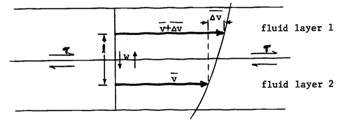
Figure 14.6: Turbulent shear stress, after Vennard and Street (1975).
Figure 14.6 represents a turbulent velocity profile, in this case for the mean horizontal velocity, as indicated by the over bar (\(\bar v\)). Notice that the portion of the profile near the lower boundary (again a flat, horizontal surface) has been omitted. This is due to the fact that in actuality a thin layer of laminar flow exists right next to the surface, which breaks down into turbulent flow immediately above. This leads to two different profile shapes, the laminar portion being omitted in Fig. 14.6 by excluding the lowest segment of the profile. (Boundary layers will be discussed in a later section; see also Monteith 1973 or Vennard and Street 1975). To visualize shearing stress for turbulent flow, we will consider the basic unit of transport to be the eddy, rather than the molecule. These eddies are randomly moving up and down between fluid layers with velocity \(w\). We will assume that an eddy moves an average distance \(l\) before it breaks up and loses its identity. (Notice the analogy here between \(l\) and mean free path of molecules.) The important point is that eddies with mean velocities of \(v\) and \(\bar v + \Delta \bar v\) are being transported up and down, carrying with them their cargoes of momentum into regions with velocities of \(\bar v + \Delta \bar v\) and \(\bar v\), respectively. This implies that momentum is exchanged between layers.
To be more explicit, consider an eddy or fluid parcel of average velocity \(\bar v\) which through turbulent motion moves up into a region of average velocity \(\bar v + \Delta \bar v\). This parcel eventually mixes with the fluid in the higher speed layer, slowing it down. The converse is true for fluid moving from regions of higher to lower velocity. The net result tends to speed up the slower layer and slow down the faster layer, which is exactly what happens in the laminar case described earlier under the action of a shearing stress. Thus we see that the existence of a shearing stress in turbulent flow can be deduced from the random motion of fluid parcels and the resultant momentum transfers (Vennard and Street 1975, p. 302 ff).
The growth and maintenance of the flow instabilities which lead to turbulent velocity fluctuations depend upon a continuous energy input. In the preceding section, it was described generally how, due to friction, energy is diverted from the mean flow to turbulent production. As a matter of fact, at the present time a fairly complete understanding of this mechanical turbulence exists. On the other hand, the energetic connection between buoyancy (convection), the other main source of turbulence, and turbulent velocity fluctuations is not nearly as well understood. The basic process involves the temperature fluctuations in the air causing corresponding density fluctuations. The result is relative motion of these different temperature air parcels, giving rise to the fluctuating velocities characteristic of turbulence. In any event, exactly how the turbulence and either the mean flow or the buoyancy are coupled energetically is beyond the scope of this treatment (see Tennekes and Lumley 1972, p. 59 ff). It must suffice at this point to state that the preceding treatment of shear flows and momentum transfer is an essential ingredient to the proper understanding of turbulent production, as well as having other important applications.