15.10 Soil Temperature
The final environmental data set in microclim is for substrate temperature. As with air temperature and relative humidity at 1cm, there are separate sets for each substrate type and shade level. Indeed, it is the thermal properties specified for each substrate type (thermal conductivity, specific heat capacity and density) that drive the substrate-specific differences in air temperature and relative humidity at 1cm. In this case we only have access to the soil substrate type.
There are 9 different depths at which soil temperature has been predicted by the microclimate model - 0, 2.5, 5, 10, 15, 20, 30, 50 and 100 cm (note the 2.5 cm layer is named 3cm, but it is for 2.5!). Let’s take a look at the 0cm depth layers in each month at midday across Australia.
month<-1 # choose which month you want, 1 or 7 (i.e. Jan or Jun)
shade <- 0 # choose which month you want, 0 or 100%
# read the file into memory
D0cm_0shade_jan<-brick(paste0(path,"substrate_temperature_degC/soil/",
                              shade,"_shade/D0cm_soil_",shade,"_",month,".nc"))

shade <- 100 # choose which month you want, 0 or 100%
# read the file into memory
D0cm_100shade_jan<-brick(paste0(path,"substrate_temperature_degC/soil/",
                                shade,"_shade/D0cm_soil_",shade,"_",month,".nc"))

month<-7 # choose which month you want, 1 or 7 (i.e. Jan or Jun)
shade <- 0 # choose which month you want, 0 or 100%
# read the file into memory
D0cm_0shade_jul<-brick(paste0(path,"substrate_temperature_degC/soil/",
                              shade,"_shade/D0cm_soil_",shade,"_",month,".nc"))

shade <- 100 # choose which month you want, 0 or 100%
# read the file into memory
D0cm_100shade_jul<-brick(paste0(path,"substrate_temperature_degC/soil/",
                                shade,"_shade/D0cm_soil_",shade,"_",month,".nc"))

par(mfrow = c(2,2)) # set to plot 2 rows of 2 panels
plot(D0cm_100shade_jan[[13]],main = "Tsoil 0cm 100% shade, 12:00 Jan, deg C", zlim = c(0,80))
plot(D0cm_100shade_jul[[13]],main = "Tsoil 0cm 100% shade, 12:00 Jul, deg C", zlim = c(0,80))
plot(D0cm_0shade_jan[[13]],main = "Tsoil 0cm 0% shade, 12:00 Jan, deg C", zlim = c(0,80))
plot(D0cm_0shade_jul[[13]],main = "Tsoil 0cm 0% shade, 12:00 Jul, deg C", zlim = c(0,80))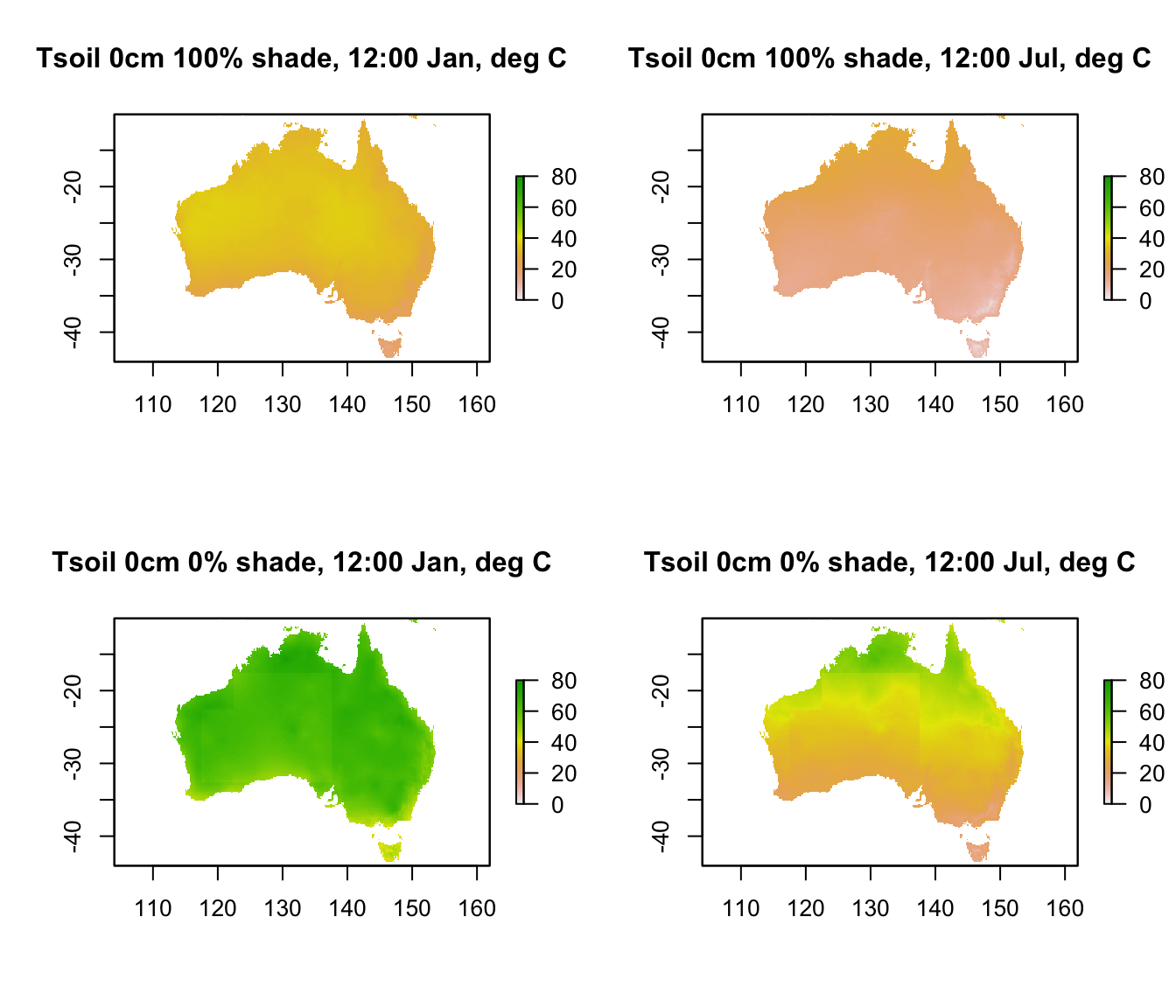
Note that there is a range of almost 80\(^\circ\)C in predicted soil surface temperature across Australia. Let’s go down 5 cm into the ground and see the difference in temperature, keeping the scale the same.
month<-1 # choose which month you want, 1 or 7 (i.e. Jan or Jun)
shade <- 0 # choose which month you want, 0 or 100%
# read the file into memory
D5cm_0shade_jan<-brick(paste0(path,"substrate_temperature_degC/soil/",
                              shade,"_shade/D5cm_soil_",shade,"_",month,".nc"))

shade <- 100 # choose which month you want, 0 or 100%
# read the file into memory
D5cm_100shade_jan<-brick(paste0(path,"substrate_temperature_degC/soil/",
                                shade,"_shade/D5cm_soil_",shade,"_",month,".nc"))

month<-7 # choose which month you want, 1 or 7 (i.e. Jan or Jun)
shade <- 0 # choose which month you want, 0 or 100%
# read the file into memory
D5cm_0shade_jul<-brick(paste0(path,"substrate_temperature_degC/soil/",
                              shade,"_shade/D5cm_soil_",shade,"_",month,".nc"))

shade <- 100 # choose which month you want, 0 or 100%
# read the file into memory
D5cm_100shade_jul<-brick(paste0(path,"substrate_temperature_degC/soil/",
                                shade,"_shade/D5cm_soil_",shade,"_",month,".nc"))

par(mfrow = c(2,2)) # set to plot 2 rows of 2 panels
plot(D5cm_100shade_jan[[13]],main = "Tsoil 5cm 100% shade, 12:00 Jan, deg C", zlim = c(0,80))
plot(D5cm_100shade_jul[[13]],main = "Tsoil 5cm 100% shade, 12:00 Jul, deg C", zlim = c(0,80))
plot(D5cm_0shade_jan[[13]],main = "Tsoil 5cm 0% shade, 12:00 Jan, deg C", zlim = c(0,80))
plot(D5cm_0shade_jul[[13]],main = "Tsoil 5cm 0% shade, 12:00 Jul, deg C", zlim = c(0,80))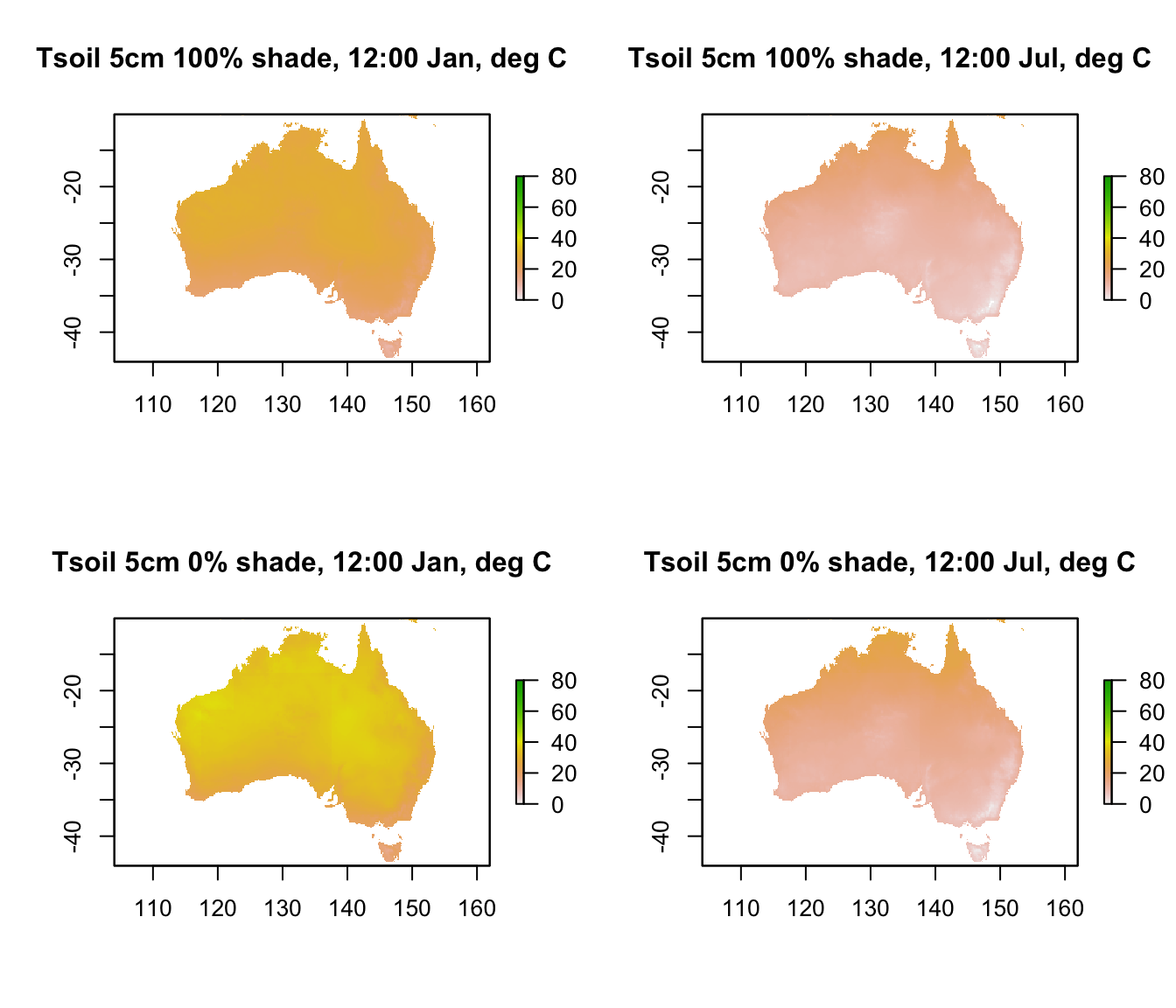
You can see that there’s a very large drop in temperature of as much as 40 degrees as you go down just 5 cm into the soil.
The next code chunk extracts the hourly temperature profile for January in 0% at the Flinders Ranges site, and then plots it
month<-1 # choose which month you want, 1 or 7 (i.e. Jan or Jun)
shade <- 0 # choose which month you want, 0 or 100%
data<-brick(paste(path,"substrate_temperature_degC/soil/",shade,
                  "_shade/D0cm_soil_",shade,"_",month,".nc",sep=""))
D0cm <- t(extract(data,lon.lat))
data<-brick(paste(path,"substrate_temperature_degC/soil/",shade,
                  "_shade/D3cm_soil_",shade,"_",month,".nc",sep=""))
D2.5cm <- t(extract(data,lon.lat))
data<-brick(paste(path,"substrate_temperature_degC/soil/",shade,
                  "_shade/D5cm_soil_",shade,"_",month,".nc",sep=""))
D5cm <- t(extract(data,lon.lat))
data<-brick(paste(path,"substrate_temperature_degC/soil/",shade,
                  "_shade/D10cm_soil_",shade,"_",month,".nc",sep=""))
D10cm <- t(extract(data,lon.lat))
data<-brick(paste(path,"substrate_temperature_degC/soil/",shade,
                  "_shade/D15cm_soil_",shade,"_",month,".nc",sep=""))
D15cm <- t(extract(data,lon.lat))
data<-brick(paste(path,"substrate_temperature_degC/soil/",shade,
                  "_shade/D20cm_soil_",shade,"_",month,".nc",sep=""))
D20cm <- t(extract(data,lon.lat))
data<-brick(paste(path,"substrate_temperature_degC/soil/",shade,
                  "_shade/D30cm_soil_",shade,"_",month,".nc",sep=""))
D30cm <- t(extract(data,lon.lat))
data<-brick(paste(path,"substrate_temperature_degC/soil/",shade,
                  "_shade/D50cm_soil_",shade,"_",month,".nc",sep=""))
D50cm <- t(extract(data,lon.lat))
data<-brick(paste(path,"substrate_temperature_degC/soil/",shade,
                  "_shade/D100cm_soil_",shade,"_",month,".nc",sep=""))
D100cm <- t(extract(data,lon.lat))

par(mfrow=c(1,1))
plot(D0cm ~ hrs,xlab = "Time of Day (hr)", ylab = "Tsoil, deg C",
     type = "l", ylim=c(0,70), main = "Soil Temperature, January")
points(D2.5cm ~ hrs,xlab = "Time of Day (hr)", col=2, type = 'l')
points(D5cm ~ hrs,xlab = "Time of Day (hr)", col=3, type = 'l')
points(D10cm ~ hrs,xlab = "Time of Day (hr)", col=4, type = 'l')
points(D15cm ~ hrs,xlab = "Time of Day (hr)", col=5, type = 'l')
points(D20cm ~ hrs,xlab = "Time of Day (hr)", col=6, type = 'l')
points(D30cm ~ hrs,xlab = "Time of Day (hr)", col=7, type = 'l')
points(D50cm ~ hrs,xlab = "Time of Day (hr)", col=8, type = 'l')
points(D100cm ~ hrs,xlab = "Time of Day (hr)",lty=2, col=9, type = 'l')

DEP <- c(0, 2.5, 5, 10, 15, 20, 30, 50, 100)
leg.txt<-paste(DEP,"cm", sep = "")
legend(1,70,lty=c(1,1,1,1,1,1,1,1,2),leg.txt,col=c(1,2,3,4,5,6,7,8,9),
       cex=1,box.lty=0)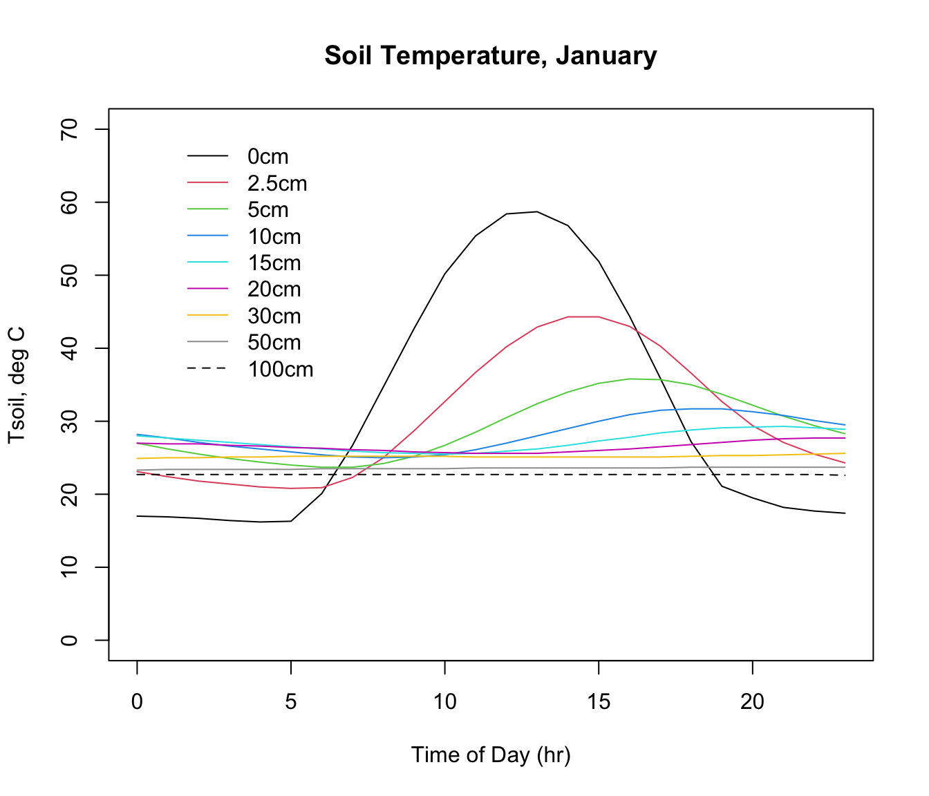
Note how the amplitude and timing of the maximum and minimum values shift with depth. The thermal profile with depth and time in the soil depends in part on the driving environmental conditions above the ground (air temperature, wind speed, radiation) but also on the thermal characteristics of the soil. This includes the moisture content, and the calculations include an estimate of soil moisture from the NOAA CPC Soil Moisture data set. The microclimate model used this soil moisture information to adjust the thermal properties of the soil at each location and month.
You can have a look at this soil temperature profile for 100% shade, or for July, by simply changing the ‘shade’ and ‘month’ values in the code chunk above. Try it, and try looking at some of these variables for other places of interest to you in Australia.