16.3 Getting the climate space available in Australia
In module 9 you recreated Figure 12 of Porter and Gates (1969) which shows the bounding combinations of radiation (solar plus infra-red) and air temperature available on earth. Recall that this was an approximation that assumed, unrealistically, that the ground temperature was equal to air temperature when computing the clear night sky bounding curve. It also attempted to capture the fact that sun angles are typically lower in the places with very low air temperatures (except for high tropical mountains), but only very roughly by assuming the zenith angle declined linearly with latitude.
Now that we have the microclim data, however, we can make a much better estimate of the bounding radiation and air temperature combinations available on earth at different times of year and at different times of day. We will do this first for Australia.
In module 9, we developed the equation Qbound. It computes the direct and diffuse radiation received by cylindrical organisms lying on the ground by a rough estimation of direct and diffuse solar radiation given the zenith angle, some parameters about the transmissivity of the atmosphere and the position of the earth in its orbit around the sun. We have this from the microclim dataset in the form of the solar radiation grids, so we can now just use them directly. These solar radiation estimates are of course already adjusted for the zenith angle and, what’s more, for variations in atmospheric transmissivity due to elevation and spatial effects (including variation in aerosols and ozone).
Our Qbound function also estimated the infra-red radiation coming down from the sky from the Swinbank formula (an empirical model) given an air temperature measured at weather station height. We can now compute this from the ‘sky temperature’ layers of the microclim data set, which inherently include the effects of cloud cover. We can also compute the infra-red radiation from the ground using the microclim substrate surface temperature estimate, rather than simply assuming ground temperature equals air temperature.
So, in summary, for our calculations of climate space boundaries from microclim we need to get the solar radiation, air temperature (we’ll choose 1cm, but we could use 120cm depending on the height of the animal of interest), substrate temperature and sky temperature. We need the latter two in the 0% shade scenario since we are interested in the extremes (what line on the climate space graph would the 100% shade scenario give us?).
We have these for January and July, which will give us the seasonal extremes. Let’s first load these layers into memory, pinching code from the previous module.
library(raster)

# put your path here for microclim data folder for Australia
path<- 'microclim_Aust/'

# read the January solar radiation file into memory
solar_jan_Aust<-brick(paste0(path,"solar_radiation_Wm2/SOLR_1.nc"))
# read the July solar radiation file into memory
solar_jul_Aust<-brick(paste0(path,"solar_radiation_Wm2/SOLR_7.nc"))
# read the January 1cm air temperature in 0% shade file into memory
Tair_jan_Aust<-brick(paste0(path,"air_temperature_degC_1cm/soil/0_shade/TA1cm_soil_0_1.nc"))
# read the July 1cm air temperature in 0% shade file into memory
Tair_jul_Aust<-brick(paste0(path,"air_temperature_degC_1cm/soil/0_shade/TA1cm_soil_0_7.nc"))
# read the January sky temperature in 0% shade file into memory
Tsky_jan_Aust<-brick(paste0(path,"sky_temperature_degC/0_shade/TSKY_0_1.nc"))
# read the January sky air temperature in 0% shade file into memory
Tsky_jul_Aust<-brick(paste0(path,"sky_temperature_degC/0_shade/TSKY_0_7.nc"))
# read the January surface temperature in 0% shade file into memory
D0cm_jan_Aust<-brick(paste0(path,"substrate_temperature_degC/soil/0_shade/D0cm_soil_0_1.nc"))
# read the July surface temperature in 0% shade file into memory
D0cm_jul_Aust<-brick(paste0(path,"substrate_temperature_degC/soil/0_shade/D0cm_soil_0_7.nc"))
Now, let’s modify the Qbound function to make it work with the grids, giving it the name Qbound_micro. Have a close look at how this differs from Qbound. Note that since we now have total solar radiation (direct plus diffuse) as an input, we need to repartition it into direct and diffuse using the parameter ‘pctdiff’ (with the value used in the original calculations for microclim, which was 15%). Air temperature is no longer an input - why? What has replaced it? Note also that we also have only one output, ‘Q_rad’, because we are making these calculations for each hour of the day so it could be for day or night.
# Computes climate space following the equations of Porter and Gates (1969),
# using the microclim layers as input

# inputs
# hg, A grid of estimated solar radiation (direct and diffuse, i.e. 'global') flux
#   on horizontal ground, W/m2
# Tsub, A grid of values (for each air temperature), of substrate temperatures, degrees C
# alpha_s, Solar absorptivity of object, decimal percent
# alpha_g, Solar absorptivity of the ground, decimal percent
# pctdiff, Proportion diffuse solar radiation, decimal percent

# outputs
# Q_rad, radiation load, W/m2

Qbound_micro <-
  function(hg = hg, Tsub = Tsub, Tsky = Tsky, alpha_s = 0.8, alpha_g = 0.8, pctdiff = 0.15) {
    sigma <- 5.670373e-8 # W/m2/k4 Stephan-Boltzman constant
    Q_ground <- (1 * sigma * (Tsub + 273.15) ^ 4) # ground radiation
    Q_sky <- (1 * sigma * (Tsky + 273.15) ^ 4) # sky thermal radiation
    hd <- hg * (1 - pctdiff) # direct solar on horizontal ground
    hS <- hg * pctdiff # diffuse (scattered) solar on horizontal ground
    r <- 1 - alpha_g # ground solar reflectance
    Q_rad <- (alpha_s * hS * (2 / pi) + alpha_s * hd + alpha_s * r * hg
              + Q_sky + Q_ground) / 2 # eq. 13 of Porter and Gates 1969
  }
Let’s now apply our function to the January data, with both our cylindrical animal and the ground having a solar absorptivity of 80%.
# getting bounding radiation conditions across Australia for January
hg = solar_jan_Aust # define the solar radiation input
Tsub = D0cm_jan_Aust # define the ground temperature input
Tsky = Tsky_jan_Aust # define the sky temperature input
alpha_s = 0.8 # animal solar absorptivity
alpha_g = 0.8 # ground solar absorptivity

# compute the total radiation load
Q_rad_jan_Aust <- Qbound_micro(hg = hg, Tsub = Tsub, Tsky = Tsky, alpha_s = alpha_s, alpha_g = alpha_g)
Now the variable ‘Q_rad’ has, for each hour of the day in January, an estimate of the total radiation load that would be present on a cylindrical animal in the open with 80% solar absorptivity. The next code chunk plots this for 4am and 12pm, together with the associated 1cm air temperatures.
par(mfrow = c(2,2)) # set to plot 2 rows of 2 panels
plot(Q_rad_jan_Aust[[5]], main = "radiation (W/m2), 4am January")
plot(Q_rad_jan_Aust[[13]], main = "radiation (W/m2), 12pm January")
plot(Tair_jan_Aust[[5]], main = "1cm air temperature (C), 4am January")
plot(Tair_jan_Aust[[13]], main = "1cm air temperature (C), 12pm January")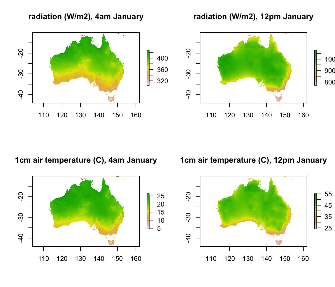
It should be clear that by projecting this data from geographic space to environmental space, i.e. to a graph of radiation vs. air temperature, we will be able to see the full range of climate space present within Australia at these times. The next code chuck creates such a graph for these two times, extracting the data from raster format into a table of values using the ‘raster’ package function values and the cbind function.
par(mfrow = c(1,1)) # revert to 1 panel
i = 5 # layer number to plot (layer 5 is 4am, because layer 1 is midnight)
# extract the radiation and air temperatures from the rasters and bind them together into a table
RadTair <- cbind(values(Q_rad_jan_Aust[[i]]),values(Tair_jan_Aust[[i]]))
plot(RadTair[,1],RadTair[,2],ylim = c(-40,60), xlim = c(0,1300), pch=16, col = 'blue',
     xlab = 'radiation, W/m2', ylab = 'air temperature, deg C',
     main = "available climate space, January")

i = 13 # layer number to plot (layer 5 is 4am, because layer 1 is midnight)
RadTair=cbind(values(Q_rad_jan_Aust[[i]]),values(Tair_jan_Aust[[i]]))
points(RadTair[,1],RadTair[,2],ylim = c(-40,60), xlim = c(0,1300), pch=16, col = 'red',
       xlab = 'radiation, W/m2', ylab = 'air temperature, deg C',
       main = "available climate space, January")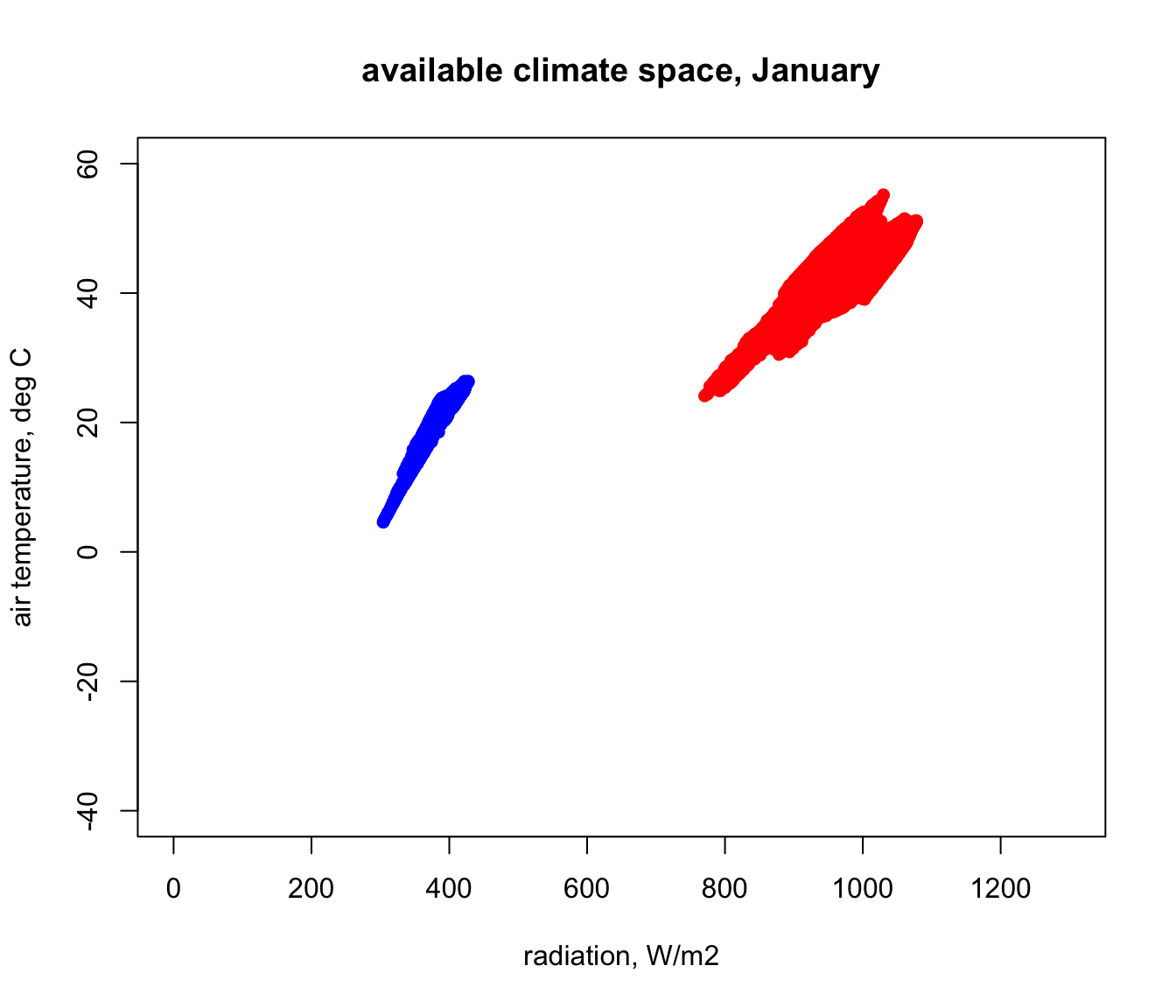
Next we will modify this code to create a loop to go through each hour, adding points to the map, for both January and July. Note that, although loops are a basic aspect of programming, they are slow in R and there are often alternatives to using them (e.g. https://www.datacamp.com/community/tutorials/tutorial-on-loops-in-r#gs.B6zaV0g).
# first, get the conditions for July
# getting bounding radiation conditions across Australia for July
hg = solar_jul_Aust # define the solar radiation input
Tsub = D0cm_jul_Aust # define the ground temperature input
Tsky = Tsky_jul_Aust # define the sky temperature input

# compute the total radiation load
Q_rad_jul_Aust <- Qbound_micro(hg = hg, Tsub = Tsub, Tsky = Tsky,
                               alpha_s = alpha_s, alpha_g = alpha_g)

# now loop through each hour and plot the results for each month
for(i in 1:24) { # start of the loop, from i = 1 to 24

  # first do January, in red
  # extract the radiation and air temperatures from the rasters and bind them together into a table
  RadTair <- cbind(values(Q_rad_jan_Aust[[i]]),values(Tair_jan_Aust[[i]]))

  if(i == 1){ # check if it is the first step, and make the first plot
    plot(RadTair[,1],RadTair[,2],ylim = c(-40,60), xlim = c(0,1300), pch = 16, col = 'red',
         xlab = 'radiation, W/m2', ylab = 'air temperature, deg C', main = "available climate space")
  }else{
    # it's not the first step, so use 'points' to add data to the plot
    points(RadTair[,1],RadTair[,2], col = 'red', pch = 16)
  } # end of the check for first plot

  # next do July, in blue
  # extract the radiation and air temperatures from the rasters and bind them together into a table
  RadTair <- cbind(values(Q_rad_jul_Aust[[i]]),values(Tair_jul_Aust[[i]]))

  # add the July values to the graph
  points(RadTair[,1],RadTair[,2], col = 'blue', pch = 16)

} # end of the loop through each hour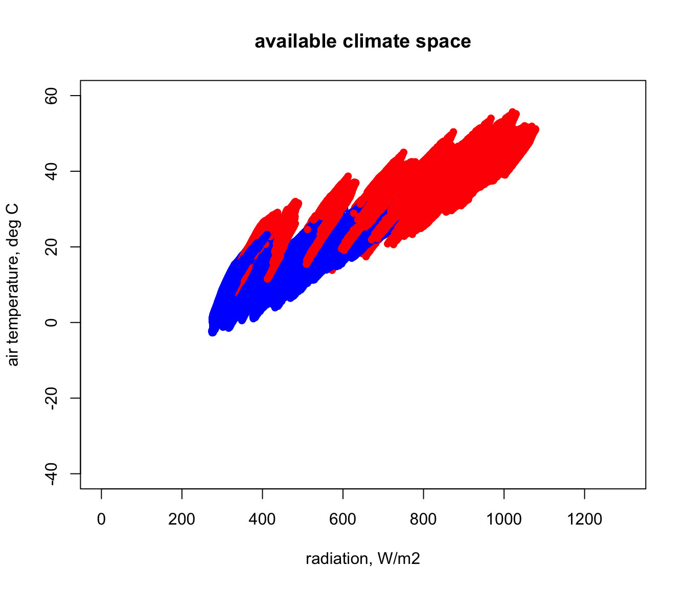
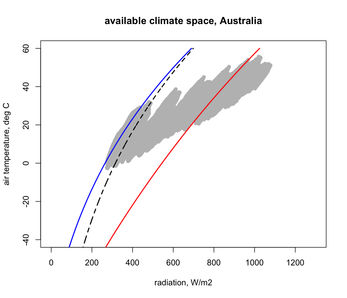
In the next figure you can see how this compares with the Figure 12 of Porter and Gates (1969). This was done by simply re-running that code and using points for the first plot to ensure that it got added onto the one we just made. How would you explain the discrepancies with our estimate for Australia using microclim?
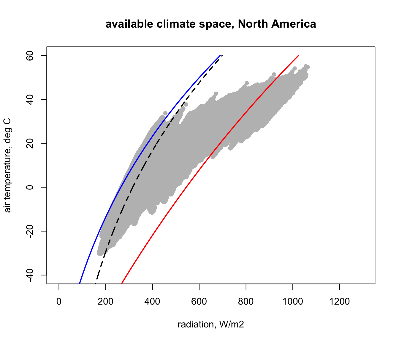
It should be an easy task to recalculate all of this for North America. Have a try, appending ‘_NAm’ to all the variables that previously had ‘_Aust’, and see if you can produce the following figure. Note how much colder it gets in North America compared with Australia.