16.4 Mapping the climate space of the Desert Iguana in North America
In module @ref(climate space) we computed the climate space of the Desert Iguana in terms of its survivable limits of 3-45 degrees C. Here are those limits for a wind speed of 0.1 m/s mapped onto our North America climate space diagram. This was done simply by using the code we developed in module @ref(climate space).
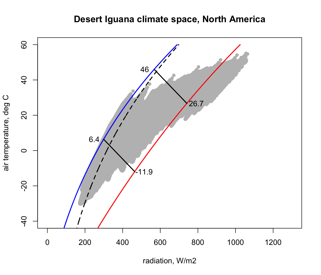
You can see that there are places within North America that are too hot and too cold for this lizard - i.e. that are outside the fundamental or ‘thermodynamic’ niche of this species with respect to temperature. We now want to see where those situations are in space and time.
To do this we can use the heat budget equation we developed in module @ref(climate space), which gives us the radiation load for a given air temperature and wind speed that would result in a particular temperature. In module @ref(climate space) we gave that equation a vector of air temperatures and a single wind speed, so we could work out those lines on the climate space diagram. But now we can give the equation grids of air temperature and wind speed and get, for each pixel, the radiation load needed to balance the heat budget at our chosen body temperature. Let’s try that now.
First, we need to define our heat budget equation as in module @ref(climate space) - remember we had one for ectotherms and one for endotherms? We need the ectotherm one of course, which has been copied and pasted here from module @ref(climate space).
# function to compute absorbed radiation required given a specific core temperature, air temperature,
# and wind speed

# organism inputs
# D, organism diameter, m
# T_b, body temperature at which calculation is to be made, deg C
# M, metabolic rate, W/m2
# E_ex, evaporative heat loss through respiration, W/m2
# E_sw, evaporative heat loss through sweating, W/m2
# K_b, thermal conductance of the skin, W/m2/C
# epsilon, emissivity of the skin, -

# environmental inputs
# Tair, A value, or vector of values, or grid of air temperatures, degrees C
# V, A value, or vector of values, or grid of wind speeds, m/s

# output
# Q_abs, predicted radiation absorbed, W/m2

Qabs_ecto <-
  function(D, T_b, M, E_ex, E_sw, K_b, epsilon, T_air, V) {
    sigma <- 5.670373e-8 # W/m2/k4 Stephan-Boltzman constant
    T_r <- T_b - (M - E_ex - E_sw) / K_b
    h_c <- 3.49 * (V^(1/2) / D^(1/2))
    Q_abs <- epsilon * sigma * (T_r + 273.15)^4 + h_c * (T_r - T_air) - M + E_ex + E_sw
    return(Q_abs)
  }
Next, we need the environmental variables for North America, including the wind speed.
# put your path here for microclim data folder for Australia
path<- 'microclim_NAm/'

# read the January wind speed file for North America into memory
wind_jan_NAm<-brick(paste0(path,"wind_speed_ms_1cm/V1cm_1.nc"))
# read the July wind speed  file for North America into memory
wind_jul_NAm<-brick(paste0(path,"wind_speed_ms_1cm/V1cm_7.nc"))
# read the January solar radiation file into memory
solar_jan_NAm<-brick(paste0(path,"solar_radiation_Wm2/SOLR_1.nc"))
# read the July solar radiation file into memory
solar_jul_NAm<-brick(paste0(path,"solar_radiation_Wm2/SOLR_7.nc"))
# read the January 1cm air temperature in 0% shade file into memory
Tair_jan_NAm<-brick(paste0(path,"air_temperature_degC_1cm/soil/0_shade/TA1cm_soil_0_1.nc"))
# read the July 1cm air temperature in 0% shade file into memory
Tair_jul_NAm<-brick(paste0(path,"air_temperature_degC_1cm/soil/0_shade/TA1cm_soil_0_7.nc"))
# read the January sky temperature in 0% shade file into memory
Tsky_jan_NAm<-brick(paste0(path,"sky_temperature_degC/0_shade/TSKY_0_1.nc"))
# read the January sky air temperature in 0% shade file into memory
Tsky_jul_NAm<-brick(paste0(path,"sky_temperature_degC/0_shade/TSKY_0_7.nc"))
# read the January surface temperature in 0% shade file into memory
D0cm_jan_NAm<-brick(paste0(path,"substrate_temperature_degC/soil/0_shade/D0cm_soil_0_1.nc"))
# read the July surface temperature in 0% shade file into memory
D0cm_jul_NAm<-brick(paste0(path,"substrate_temperature_degC/soil/0_shade/D0cm_soil_0_7.nc"))
We have the environmental variables; now we need the organism’s parameters. As in module @ref(climate space), we read in the climate space parameters ‘csv’ file, subset it for the Desert Iguana data, and convert to SI units where necessary.
climate_space_pars <- as.data.frame(read.csv("data/climate_space_pars.csv"))
pars <- subset(climate_space_pars, Name=="Desert Iguana")
# convert heat flows from cal/min/cm2 to J/s/m2 = W/m2
pars[,4:6] <- pars[,4:6] * (4.185 / 60 * 10000)
# convert thermal conductivities from cal/(min cm C) to J/(s m C) = W/(m C)
pars[,14:15] <- pars[,14:15] * (4.185 / 60 * 100)
pars[,c(7:8,11,16)] <- pars[,c(7:8,11,16)] / 100 # convert cm to m