22.5 Shopping carts analysis
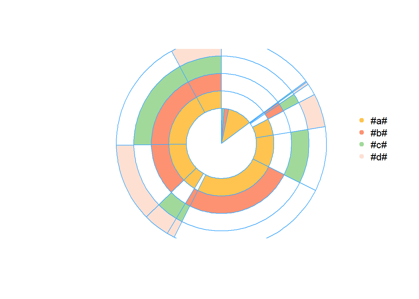
22.5.1 Multi-layer pie chart
Example by Sergey Bryl
# loading libraries
library(dplyr)
library(tidyverse)
library(reshape2)
library(plotrix)

# Simulate of orders
set.seed(15)
df <- data.frame(
    orderId = sample(c(1:1000), 5000, replace = TRUE),
    product = sample(
        c('NULL', 'a', 'b', 'c', 'd'),
        5000,
        replace = TRUE,
        prob = c(0.15, 0.65, 0.3, 0.15, 0.1)
    )
)
df <- df[df$product != 'NULL',]
head(df)
## orderId product
## 1 549 b
## 3 874 a
## 4 674 d
## 5 505 a
## 6 294 a
## 7 177 a# processing initial data
# we need to be sure that product's names are unique
df$product <- paste0("#", df$product, "#")
prod.matrix <- df %>%
# removing duplicated products from each order (exclude the effect of quantity)
group_by(orderId, product) %>%
arrange(product) %>%
unique() %>%
# combining products to cart and calculating number of products
group_by(orderId) %>%
summarise(cart = paste(product, collapse = ";"),
prod.num = n()) %>%
# calculating number of carts
group_by(cart, prod.num) %>%
summarise(num = n()) %>%
ungroup()
head(prod.matrix)## # A tibble: 6 × 3
## cart prod.num num
## <chr> <int> <int>
## 1 #a# 1 115
## 2 #a#;#b# 2 248
## 3 #a#;#b#;#c# 3 172
## 4 #a#;#b#;#c#;#d# 4 78
## 5 #a#;#b#;#d# 3 119
## 6 #a#;#c# 2 98# calculating total number of orders/carts
tot <- sum(prod.matrix$num)
# spliting orders for sets with 1 product and more than 1 product
one.prod <- prod.matrix %>% filter(prod.num == 1)
sev.prod <- prod.matrix %>%
filter(prod.num > 1) %>%
arrange(desc(prod.num))# defining parameters for pie chart
iniR <- 0.2 # initial radius
cols <- c(
"#ffffff",
"#fec44f",
"#fc9272",
"#a1d99b",
"#fee0d2",
"#2ca25f",
"#8856a7",
"#43a2ca",
"#fdbb84",
"#e34a33",
"#a6bddb",
"#dd1c77",
"#ffeda0",
"#756bb1"
)
prod <- df %>%
select(product) %>%
arrange(product) %>%
unique()
prod <- c('NO', c(prod$product))
colors <- as.list(setNames(cols[c(1:(length(prod)))], prod))# 0 circle: blank
pie(
1,
radius = iniR,
init.angle = 90,
col = c('white'),
border = NA,
labels = ''
)
# drawing circles from last to 2nd
for (i in length(prod):2) {
p <- grep(prod[i], sev.prod$cart)
col <- rep('NO', times = nrow(sev.prod))
col[p] <- prod[i]
floating.pie(
0,
0,
c(sev.prod$num, tot - sum(sev.prod$num)),
radius = (1 + i) * iniR,
startpos = pi / 2,
col = as.character(colors [c(col, 'NO')]),
border = "#44aaff"
)
}
# 1 circle: orders with 1 product
floating.pie(
0,
0,
c(tot - sum(one.prod$num), one.prod$num),
radius = 2 * iniR,
startpos = pi / 2,
col = as.character(colors [c('NO', one.prod$cart)]),
border = "#44aaff"
)
# legend
legend(
1.5,
2 * iniR,
gsub("_", " ", names(colors)[-1]),
col = as.character(colors [-1]),
pch = 19,
bty = 'n',
ncol = 1
)
# creating a table with the stats
stat.tab <- prod.matrix %>%
    select(-prod.num) %>%
    mutate(share = num / tot) %>%
    arrange(desc(num))

library(scales)
stat.tab$share <-
    percent(stat.tab$share) # converting values to percents

# adding a table with the stats
# addtable2plot(
#     -2.5,
#     -1.5,
#     stat.tab,
#     bty = "n",
#     display.rownames = FALSE,
#     hlines = FALSE,
#     vlines = FALSE,
#     title = "The stats"
# )
22.5.2 Sankey Diagram
# loading libraries
library(googleVis)
library(dplyr)
library(reshape2)

# creating an example of orders
set.seed(15)
df <- data.frame(
    orderId = c(1:1000),
    clientId = sample(c(1:300), 1000, replace = TRUE),
    prod1 = sample(
        c('NULL', 'a'),
        1000,
        replace = TRUE,
        prob = c(0.15, 0.5)
    ),
    prod2 = sample(
        c('NULL', 'b'),
        1000,
        replace = TRUE,
        prob = c(0.15, 0.3)
    ),
    prod3 = sample(
        c('NULL', 'c'),
        1000,
        replace = TRUE,
        prob = c(0.15, 0.2)
    )
)

# combining products
df$cart <- paste(df$prod1, df$prod2, df$prod3, sep = ';')
df$cart <- gsub('NULL;|;NULL', '', df$cart)
df <- df[df$cart != 'NULL',]

df <- df %>%
    select(orderId, clientId, cart) %>%
    arrange(clientId, orderId, cart)

head(df)
## orderId clientId cart
## 1 181 1 b
## 2 282 1 a
## 3 748 1 a;b;c
## 4 27 2 a;b
## 5 209 2 b;c
## 6 244 2 a;b;corders <- df %>%
group_by(clientId) %>%
mutate(n.ord = paste('ord', c(1:n()), sep = '')) %>%
ungroup()
head(orders)## # A tibble: 6 × 4
## orderId clientId cart n.ord
## <int> <int> <chr> <chr>
## 1 181 1 b ord1
## 2 282 1 a ord2
## 3 748 1 a;b;c ord3
## 4 27 2 a;b ord1
## 5 209 2 b;c ord2
## 6 244 2 a;b;c ord3orders <-
dcast(orders,
clientId ~ n.ord,
value.var = 'cart',
fun.aggregate = NULL)
# choose a number of carts/orders in the sequence we want to analyze
orders <- orders %>%
select(ord1, ord2, ord3, ord4, ord5)
orders.plot <- data.frame()
for (i in 2:ncol(orders)) {
ord.cache <- orders %>%
group_by(orders[, i - 1], orders[, i]) %>%
summarise(n = n()) %>%
ungroup()
colnames(ord.cache)[1:2] <- c('from', 'to')
# adding tags to carts
ord.cache$from <- paste(ord.cache$from, '(', i - 1, ')', sep = '')
ord.cache$to <- paste(ord.cache$to, '(', i, ')', sep = '')
orders.plot <- rbind(orders.plot, ord.cache)
}
plot(gvisSankey(
orders.plot,
from = 'from',
to = 'to',
weight = 'n',
options = list(
height = 900,
width = 1800,
sankey = "{link:{color:{fill:'lightblue'}}}"
)
))
# The bandwidths correspond to the weight of sequence22.5.3 Sequence in-depth analysis
Example by Sergey Bryl
To understand customer’s behavior and churn based on purchase sequence. For example,
If the customer has left or did not make the next purchase
Understand duration between purchases
library(dplyr)
library(TraMineR)
library(reshape2)
library(googleVis)

# creating an example of shopping carts
set.seed(10)
data <- data.frame(
    orderId = sample(c(1:1000), 5000, replace = TRUE),
    product = sample(
        c('NULL', 'a', 'b', 'c'), # assume we have only 3 products
        5000,
        replace = TRUE,
        prob = c(0.15, 0.65, 0.3, 0.15)
    )
)

# we also know customers' purchase order
order <- data.frame(orderId = c(1:1000),
                    clientId = sample(c(1:300), 1000, replace = TRUE))

# suppose we know customers' gender
sex <- data.frame(clientId = c(1:300),
                  sex = sample(
                      c('male', 'female'),
                      300,
                      replace = TRUE,
                      prob = c(0.40, 0.60)
                  ))


date <- data.frame(orderId = c(1:1000),
                   orderdate = sample((1:90), 1000, replace = TRUE))
orders <- merge(data, order, by = 'orderId')
orders <- merge(orders, sex, by = 'clientId')
orders <- merge(orders, date, by = 'orderId')
orders <- orders[orders$product != 'NULL',]
orders$orderdate <- as.Date(orders$orderdate, origin = "2012-01-01")
rm(data, date, order, sex)

head(orders)
## orderId clientId product sex orderdate
## 1 1 204 a female 2012-02-11
## 2 1 204 a female 2012-02-11
## 3 1 204 a female 2012-02-11
## 4 1 204 a female 2012-02-11
## 5 2 71 a male 2012-02-27
## 6 2 71 a male 2012-02-27# combining products to the cart (include cases where customers make 2 visits in a day)
df <- orders %>%
arrange(product) %>%
select(-orderId) %>%
unique() %>%
group_by(clientId, sex, orderdate) %>%
summarise(cart = paste(product, collapse = ";")) %>%
ungroup()
head(df)## # A tibble: 6 × 4
## clientId sex orderdate cart
## <int> <chr> <date> <chr>
## 1 1 female 2012-02-18 a;c
## 2 1 female 2012-03-19 a;b;c
## 3 1 female 2012-03-21 a;b;c
## 4 2 female 2012-02-14 a;b
## 5 2 female 2012-02-27 a;b
## 6 2 female 2012-03-06 amax.date <- max(df$orderdate) + 1
ids <- unique(df$clientId)
df.new <- data.frame()
for (i in 1:length(ids)) {
df.cache <- df %>%
filter(clientId == ids[i])
ifelse(nrow(df.cache) == 1,
av.dur <- 30,
av.dur <-
round(((
max(df.cache$orderdate) - min(df.cache$orderdate)
) / (
nrow(df.cache) - 1
)) * 1.5, 0))
df.cache <-
rbind(
df.cache,
data.frame(
clientId = df.cache$clientId[nrow(df.cache)],
sex = df.cache$sex[nrow(df.cache)],
orderdate = max(df.cache$orderdate) + av.dur,
cart = 'nopurch'
)
)
ifelse(max(df.cache$orderdate) > max.date,
df.cache$orderdate[which.max(df.cache$orderdate)] <- max.date,
NA)
df.cache$to <- c(df.cache$orderdate[2:nrow(df.cache)] - 1, max.date)
# order# for Sankey diagram
df.cache <- df.cache %>%
mutate(ord = paste('ord', c(1:nrow(df.cache)), sep = ''))
df.new <- rbind(df.new, df.cache)
}
# filtering dummies
df.new <- df.new %>%
filter(cart != 'nopurch' | to != orderdate)
rm(orders, df, df.cache, i, ids, max.date, av.dur)
##### Sankey diagram #######
df.sankey <- df.new %>%
select(clientId, cart, ord)
df.sankey <-
dcast(df.sankey,
clientId ~ ord,
value.var = 'cart',
fun.aggregate = NULL)
df.sankey[is.na(df.sankey)] <- 'unknown'
# chosing a length of sequence
df.sankey <- df.sankey %>%
select(ord1, ord2, ord3, ord4)
# replacing NAs after 'nopurch' for 'nopurch'
df.sankey[df.sankey[, 2] == 'nopurch', 3] <- 'nopurch'
df.sankey[df.sankey[, 3] == 'nopurch', 4] <- 'nopurch'
df.sankey.plot <- data.frame()
for (i in 2:ncol(df.sankey)) {
df.sankey.cache <- df.sankey %>%
group_by(df.sankey[, i - 1], df.sankey[, i]) %>%
summarise(n = n()) %>%
ungroup()
colnames(df.sankey.cache)[1:2] <- c('from', 'to')
# adding tags to carts
df.sankey.cache$from <-
paste(df.sankey.cache$from, '(', i - 1, ')', sep = '')
df.sankey.cache$to <- paste(df.sankey.cache$to, '(', i, ')', sep = '')
df.sankey.plot <- rbind(df.sankey.plot, df.sankey.cache)
}
plot(gvisSankey(
df.sankey.plot,
from = 'from',
to = 'to',
weight = 'n',
options = list(
height = 900,
width = 1800,
sankey = "{link:{color:{fill:'lightblue'}}}"
)
))
rm(df.sankey, df.sankey.cache, df.sankey.plot, i)
df.new <- df.new %>%
# chosing a length of sequence
filter(ord %in% c('ord1', 'ord2', 'ord3', 'ord4')) %>%
select(-ord)
# converting dates to numbers
min.date <- as.Date(min(df.new$orderdate), format = "%Y-%m-%d")
df.new$orderdate <- as.numeric(df.new$orderdate - min.date + 1)
df.new$to <- as.numeric(df.new$to - min.date + 1)
df.form <-
seqformat(
as.data.frame(df.new),
id = 'clientId',
begin = 'orderdate',
end = 'to',
status = 'cart',
from = 'SPELL',
to = 'STS',
process = FALSE
)
df.seq <-
seqdef(df.form,
left = 'DEL',
right = 'unknown',
xtstep = 10) # xtstep - step between ticks (days)
summary(df.seq)## [>] sequence object created with TraMineR version 2.2-7
## [>] 288 sequences in the data set, 286 unique
## [>] min/max sequence length: 4/91
## [>] alphabet (state labels):
## 1=a (a)
## 2=a;b (a;b)
## 3=a;b;c (a;b;c)
## 4=a;c (a;c)
## 5=b (b)
## 6=b;c (b;c)
## 7=c (c)
## 8=nopurch (nopurch)
## 9=unknown (unknown)
## [>] dimensionality of the sequence space: 728
## [>] colors: 1=#8DD3C7 2=#FFFFB3 3=#BEBADA 4=#FB8072 5=#80B1D3 6=#FDB462 7=#B3DE69 8=#FCCDE5 9=#D9D9D9
## [>] symbol for void element: %df.feat <- unique(df.new[, c('clientId', 'sex')])
# distribution analysis
seqdplot(df.seq, border = NA, withlegend = 'right')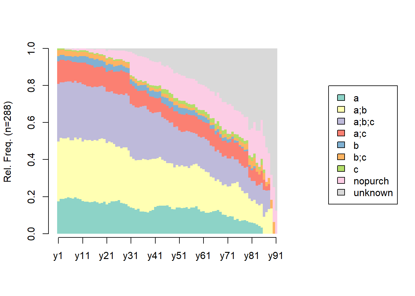
##               [State frequencies]
##            y1     y2     y3     y4     y5    y6     y7    y8     y9   y10   y11
## a       0.174 0.1875 0.1875 0.1910 0.1951 0.192 0.1888 0.196 0.1895 0.187 0.176
## a;b     0.323 0.3299 0.3264 0.3229 0.3240 0.311 0.3147 0.323 0.3193 0.331 0.320
## a;b;c   0.312 0.2986 0.3021 0.3056 0.3031 0.318 0.3112 0.305 0.3053 0.299 0.310
## a;c     0.122 0.1215 0.1215 0.1146 0.1150 0.112 0.1119 0.102 0.1088 0.106 0.116
## b       0.028 0.0278 0.0278 0.0243 0.0209 0.024 0.0280 0.032 0.0316 0.035 0.035
## b;c     0.031 0.0278 0.0278 0.0278 0.0279 0.028 0.0280 0.025 0.0246 0.025 0.025
## c       0.010 0.0069 0.0069 0.0069 0.0070 0.007 0.0070 0.007 0.0070 0.007 0.007
## nopurch 0.000 0.0000 0.0000 0.0035 0.0035 0.007 0.0070 0.011 0.0105 0.011 0.011
## unknown 0.000 0.0000 0.0000 0.0035 0.0035 0.000 0.0035 0.000 0.0035 0.000 0.000
##           y12    y13    y14    y15    y16    y17    y18    y19    y20    y21
## a       0.173 0.1725 0.1696 0.1702 0.1744 0.1685 0.1619 0.1655 0.1727 0.1583
## a;b     0.335 0.3310 0.3357 0.3298 0.3310 0.3333 0.3489 0.3489 0.3381 0.3309
## a;b;c   0.296 0.2923 0.2898 0.2908 0.2883 0.2903 0.2842 0.2842 0.2806 0.2770
## a;c     0.120 0.1197 0.1166 0.1170 0.1032 0.1075 0.1043 0.1043 0.1043 0.1079
## b       0.035 0.0387 0.0353 0.0390 0.0427 0.0430 0.0360 0.0324 0.0324 0.0360
## b;c     0.025 0.0246 0.0247 0.0248 0.0249 0.0251 0.0252 0.0252 0.0288 0.0288
## c       0.007 0.0070 0.0071 0.0071 0.0071 0.0072 0.0072 0.0072 0.0072 0.0072
## nopurch 0.011 0.0106 0.0177 0.0177 0.0214 0.0215 0.0288 0.0288 0.0324 0.0396
## unknown 0.000 0.0035 0.0035 0.0035 0.0071 0.0036 0.0036 0.0036 0.0036 0.0144
##            y22    y23    y24    y25    y26    y27    y28    y29    y30    y31
## a       0.1667 0.1739 0.1745 0.1758 0.1801 0.1661 0.1624 0.1587 0.1481 0.1407
## a;b     0.3297 0.3188 0.3091 0.2930 0.2904 0.2952 0.3026 0.3063 0.3000 0.2741
## a;b;c   0.2681 0.2754 0.2727 0.2857 0.2794 0.2915 0.2841 0.2915 0.2963 0.2852
## a;c     0.1159 0.1159 0.1164 0.1209 0.1250 0.1292 0.1255 0.1144 0.1222 0.1074
## b       0.0362 0.0290 0.0291 0.0293 0.0331 0.0295 0.0295 0.0258 0.0259 0.0259
## b;c     0.0290 0.0290 0.0291 0.0293 0.0257 0.0258 0.0258 0.0258 0.0259 0.0148
## c       0.0072 0.0072 0.0073 0.0073 0.0074 0.0037 0.0037 0.0037 0.0074 0.0074
## nopurch 0.0399 0.0399 0.0509 0.0476 0.0478 0.0480 0.0554 0.0590 0.0556 0.1259
## unknown 0.0072 0.0109 0.0109 0.0110 0.0110 0.0111 0.0111 0.0148 0.0185 0.0185
##            y32    y33    y34    y35    y36    y37   y38   y39   y40   y41   y42
## a       0.1370 0.1296 0.1338 0.1199 0.1199 0.1170 0.114 0.122 0.127 0.144 0.149
## a;b     0.2667 0.2667 0.2639 0.2772 0.2846 0.2830 0.284 0.279 0.277 0.261 0.259
## a;b;c   0.2889 0.2852 0.2825 0.2884 0.2846 0.2906 0.273 0.256 0.246 0.249 0.247
## a;c     0.1037 0.1000 0.0892 0.0861 0.0824 0.0830 0.087 0.084 0.088 0.078 0.075
## b       0.0259 0.0296 0.0297 0.0300 0.0300 0.0302 0.030 0.031 0.035 0.035 0.035
## b;c     0.0185 0.0185 0.0186 0.0187 0.0112 0.0113 0.011 0.019 0.015 0.016 0.016
## c       0.0074 0.0074 0.0074 0.0075 0.0075 0.0075 0.011 0.011 0.012 0.016 0.016
## nopurch 0.1259 0.1296 0.1338 0.1311 0.1348 0.1283 0.136 0.134 0.131 0.128 0.129
## unknown 0.0259 0.0333 0.0409 0.0412 0.0449 0.0491 0.053 0.065 0.069 0.074 0.075
##           y43   y44   y45   y46   y47   y48   y49   y50   y51   y52   y53   y54
## a       0.151 0.151 0.151 0.153 0.145 0.133 0.130 0.140 0.140 0.137 0.140 0.142
## a;b     0.263 0.247 0.241 0.227 0.236 0.246 0.227 0.230 0.221 0.232 0.223 0.222
## a;b;c   0.243 0.231 0.229 0.231 0.219 0.221 0.218 0.209 0.196 0.180 0.188 0.191
## a;c     0.076 0.076 0.078 0.079 0.079 0.083 0.084 0.081 0.089 0.094 0.092 0.093
## b       0.036 0.036 0.037 0.041 0.037 0.029 0.034 0.034 0.034 0.034 0.035 0.027
## b;c     0.016 0.016 0.020 0.021 0.021 0.021 0.021 0.021 0.021 0.021 0.022 0.013
## c       0.016 0.024 0.024 0.025 0.025 0.021 0.017 0.017 0.017 0.017 0.017 0.018
## nopurch 0.127 0.127 0.122 0.132 0.136 0.133 0.134 0.136 0.140 0.137 0.135 0.133
## unknown 0.072 0.092 0.098 0.091 0.103 0.112 0.134 0.132 0.140 0.146 0.148 0.160
##           y55   y56   y57    y58    y59    y60   y61    y62    y63   y64   y65
## a       0.135 0.140 0.142 0.1475 0.1308 0.1190 0.121 0.1127 0.1133 0.116 0.122
## a;b     0.220 0.226 0.233 0.2304 0.2336 0.2333 0.227 0.2206 0.2167 0.192 0.180
## a;b;c   0.197 0.181 0.169 0.1613 0.1589 0.1667 0.174 0.1765 0.1724 0.167 0.169
## a;c     0.090 0.090 0.096 0.0922 0.0935 0.0952 0.082 0.0882 0.0936 0.091 0.095
## b       0.027 0.027 0.027 0.0230 0.0234 0.0238 0.029 0.0294 0.0197 0.020 0.021
## b;c     0.013 0.014 0.014 0.0092 0.0093 0.0095 0.014 0.0098 0.0099 0.015 0.011
## c       0.018 0.018 0.018 0.0184 0.0187 0.0190 0.019 0.0196 0.0197 0.020 0.026
## nopurch 0.139 0.140 0.137 0.1429 0.1402 0.1381 0.135 0.1373 0.1379 0.146 0.143
## unknown 0.161 0.163 0.164 0.1751 0.1916 0.1952 0.198 0.2059 0.2167 0.232 0.233
##           y66   y67   y68   y69   y70   y71   y72   y73   y74    y75    y76
## a       0.123 0.127 0.117 0.102 0.101 0.091 0.094 0.093 0.075 0.0786 0.0682
## a;b     0.160 0.166 0.162 0.159 0.166 0.164 0.163 0.179 0.197 0.2000 0.1818
## a;b;c   0.160 0.160 0.156 0.153 0.154 0.152 0.150 0.146 0.129 0.1214 0.1288
## a;c     0.091 0.094 0.084 0.085 0.083 0.085 0.087 0.093 0.088 0.0929 0.0909
## b       0.021 0.017 0.017 0.017 0.018 0.018 0.019 0.013 0.014 0.0071 0.0076
## b;c     0.011 0.017 0.017 0.017 0.018 0.012 0.012 0.013 0.014 0.0143 0.0227
## c       0.027 0.028 0.028 0.023 0.024 0.018 0.012 0.013 0.020 0.0214 0.0227
## nopurch 0.150 0.155 0.151 0.153 0.148 0.158 0.163 0.139 0.129 0.1286 0.1364
## unknown 0.257 0.238 0.268 0.290 0.290 0.303 0.300 0.311 0.333 0.3357 0.3409
##            y77    y78    y79    y80    y81   y82   y83   y84   y85   y86   y87
## a       0.0714 0.0726 0.0672 0.0603 0.0588 0.057 0.049 0.042 0.032 0.000 0.000
## a;b     0.1587 0.1452 0.1513 0.1293 0.1176 0.125 0.111 0.111 0.129 0.091 0.116
## a;b;c   0.1349 0.1371 0.1429 0.1121 0.1078 0.102 0.099 0.111 0.113 0.145 0.116
## a;c     0.0952 0.0887 0.0840 0.0603 0.0588 0.068 0.074 0.056 0.065 0.055 0.023
## b       0.0079 0.0081 0.0084 0.0086 0.0098 0.011 0.000 0.000 0.000 0.000 0.000
## b;c     0.0238 0.0323 0.0336 0.0345 0.0392 0.045 0.037 0.028 0.032 0.036 0.023
## c       0.0238 0.0161 0.0168 0.0172 0.0196 0.023 0.012 0.014 0.032 0.018 0.000
## nopurch 0.1270 0.1290 0.1261 0.1379 0.1569 0.170 0.173 0.194 0.210 0.182 0.186
## unknown 0.3571 0.3710 0.3697 0.4397 0.4314 0.398 0.444 0.444 0.387 0.473 0.535
##           y88   y89   y90  y91
## a       0.000 0.000 0.000 0.00
## a;b     0.133 0.136 0.000 0.00
## a;b;c   0.100 0.000 0.000 0.00
## a;c     0.033 0.000 0.000 0.00
## b       0.000 0.000 0.000 0.00
## b;c     0.033 0.045 0.062 0.00
## c       0.000 0.000 0.000 0.00
## nopurch 0.133 0.136 0.188 0.12
## unknown 0.567 0.682 0.750 0.88
##
##                [Valid states]
##          y1  y2  y3  y4  y5  y6  y7  y8  y9 y10 y11 y12 y13 y14 y15 y16 y17 y18
## N       288 288 288 288 287 286 286 285 285 284 284 284 284 283 282 281 279 278
##         y19 y20 y21 y22 y23 y24 y25 y26 y27 y28 y29 y30 y31 y32 y33 y34 y35 y36
## N       278 278 278 276 276 275 273 272 271 271 271 270 270 270 270 269 267 267
##         y37 y38 y39 y40 y41 y42 y43 y44 y45 y46 y47 y48 y49 y50 y51 y52 y53 y54
## N       265 264 262 260 257 255 251 251 245 242 242 240 238 235 235 233 229 225
##         y55 y56 y57 y58 y59 y60 y61 y62 y63 y64 y65 y66 y67 y68 y69 y70 y71 y72
## N       223 221 219 217 214 210 207 204 203 198 189 187 181 179 176 169 165 160
##         y73 y74 y75 y76 y77 y78 y79 y80 y81 y82 y83 y84 y85 y86 y87 y88 y89 y90
## N       151 147 140 132 126 124 119 116 102  88  81  72  62  55  43  30  22  16
##         y91
## N         8
##
##                [Entropy index]
##          y1  y2  y3   y4   y5   y6   y7   y8   y9  y10  y11  y12  y13  y14  y15
## H       0.7 0.7 0.7 0.71 0.71 0.71 0.72 0.71 0.72 0.71 0.72 0.72 0.73 0.73 0.74
##          y16  y17  y18  y19  y20  y21  y22  y23  y24  y25  y26  y27  y28  y29
## H       0.75 0.74 0.74 0.74 0.75 0.77 0.77 0.77 0.78 0.78 0.78 0.77 0.78 0.77
##          y30 y31  y32  y33  y34  y35  y36  y37  y38  y39  y40  y41  y42  y43
## H       0.78 0.8 0.81 0.82 0.82 0.82 0.81 0.81 0.82 0.84 0.85 0.85 0.86 0.86
##          y44  y45  y46  y47  y48  y49  y50  y51  y52 y53  y54  y55  y56  y57
## H       0.87 0.88 0.89 0.89 0.88 0.89 0.89 0.89 0.89 0.9 0.88 0.88 0.88 0.88
##          y58  y59  y60  y61  y62  y63  y64  y65  y66  y67  y68  y69  y70  y71
## H       0.87 0.87 0.87 0.88 0.88 0.87 0.88 0.88 0.88 0.88 0.87 0.86 0.86 0.85
##          y72  y73  y74  y75  y76  y77  y78  y79  y80  y81  y82  y83  y84  y85
## H       0.84 0.84 0.83 0.82 0.83 0.83 0.82 0.82 0.78 0.79 0.81 0.75 0.74 0.78
##          y86 y87 y88  y89  y90  y91
## H       0.69 0.6 0.6 0.43 0.32 0.17
df.seq <- seqdef(df.form,
left = 'DEL',
right = 'DEL',
xtstep = 10)
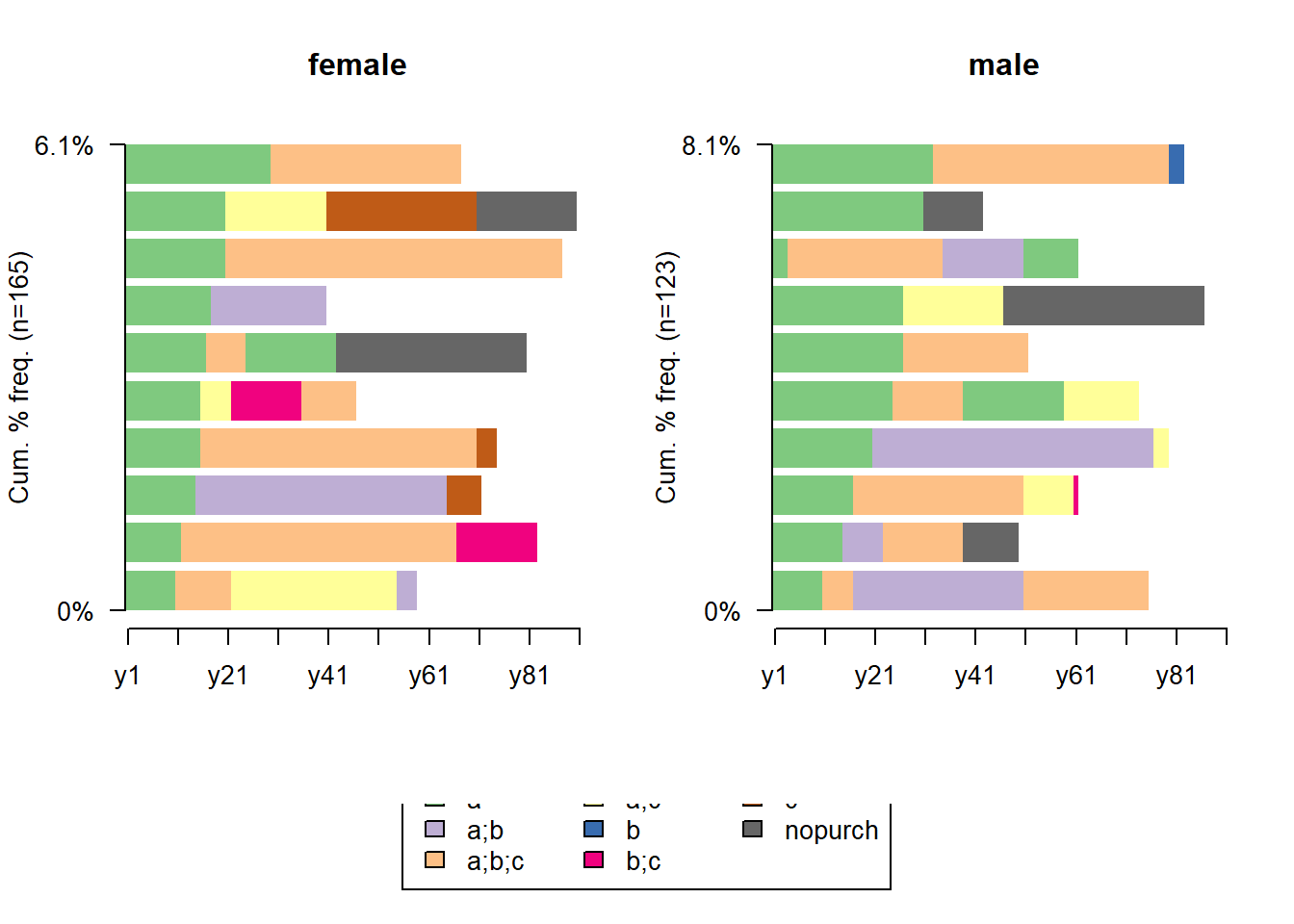
# the 10 most frequent sequences
seqfplot(df.seq, border = NA, withlegend = 'right')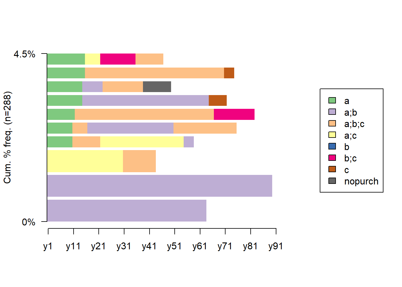
##                                Freq Percent
## a;b/63                            2    0.69
## a;b/89                            2    0.69
## a;c/30-a;b;c/13                   2    0.69
## a/10-a;b;c/11-a;c/33-a;b/4        1    0.35
## a/10-a;b;c/6-a;b/34-a;b;c/25      1    0.35
## a/11-a;b;c/55-b;c/16              1    0.35
## a/14-a;b/50-c/7                   1    0.35
## a/14-a;b/8-a;b;c/16-nopurch/11    1    0.35
## a/15-a;b;c/55-c/4                 1    0.35
## a/15-a;c/6-b;c/14-a;b;c/11 1 0.35## Freq Percent
## a;b;c/30 41 14.24
## a;b/30 40 13.89
## a/30 24 8.33
## a;c/30 15 5.21
## b;c/30 4 1.39
## a;b/1-a;b;c/29 2 0.69
## a;b;c/28-a;b/2 2 0.69
## a;c/15-a;b/15 2 0.69
## a;c/7-a;b/23 2 0.69
## b/30 2 0.69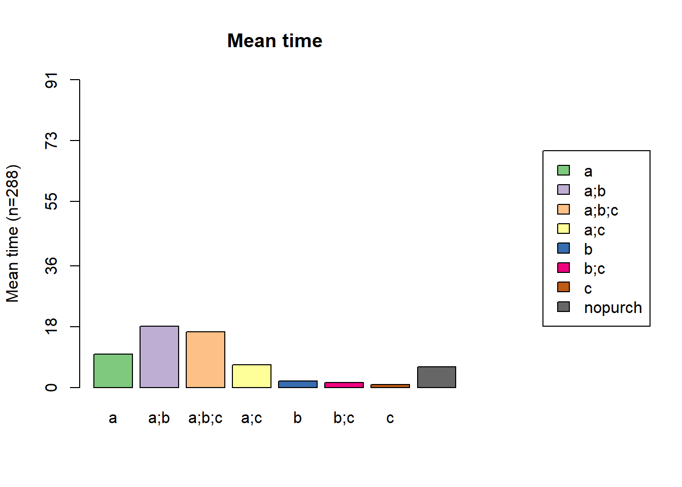
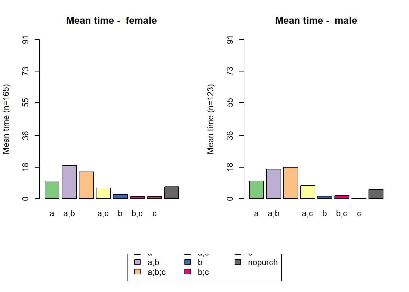
statd <-
    seqistatd(df.seq) #function returns for each sequence the time spent in the different states
apply(statd, 2, mean) #We may be interested in the mean time spent in each state
## a a;b a;b;c a;c b b;c c
## 9.7916667 18.0416667 16.4201389 6.6840278 1.9236111 1.4583333 0.8611111
## nopurch
## 6.0694444# calculating entropy
df.ient <- seqient(df.seq)
hist(df.ient,
col = 'cyan',
main = NULL,
xlab = 'Entropy') # plot an histogram of the within entropy of the sequences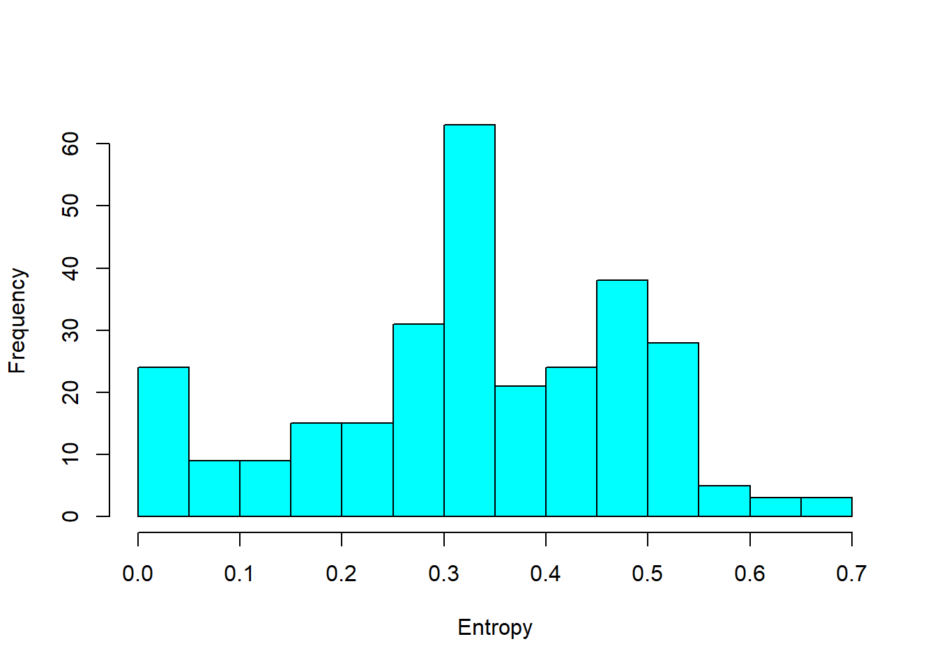
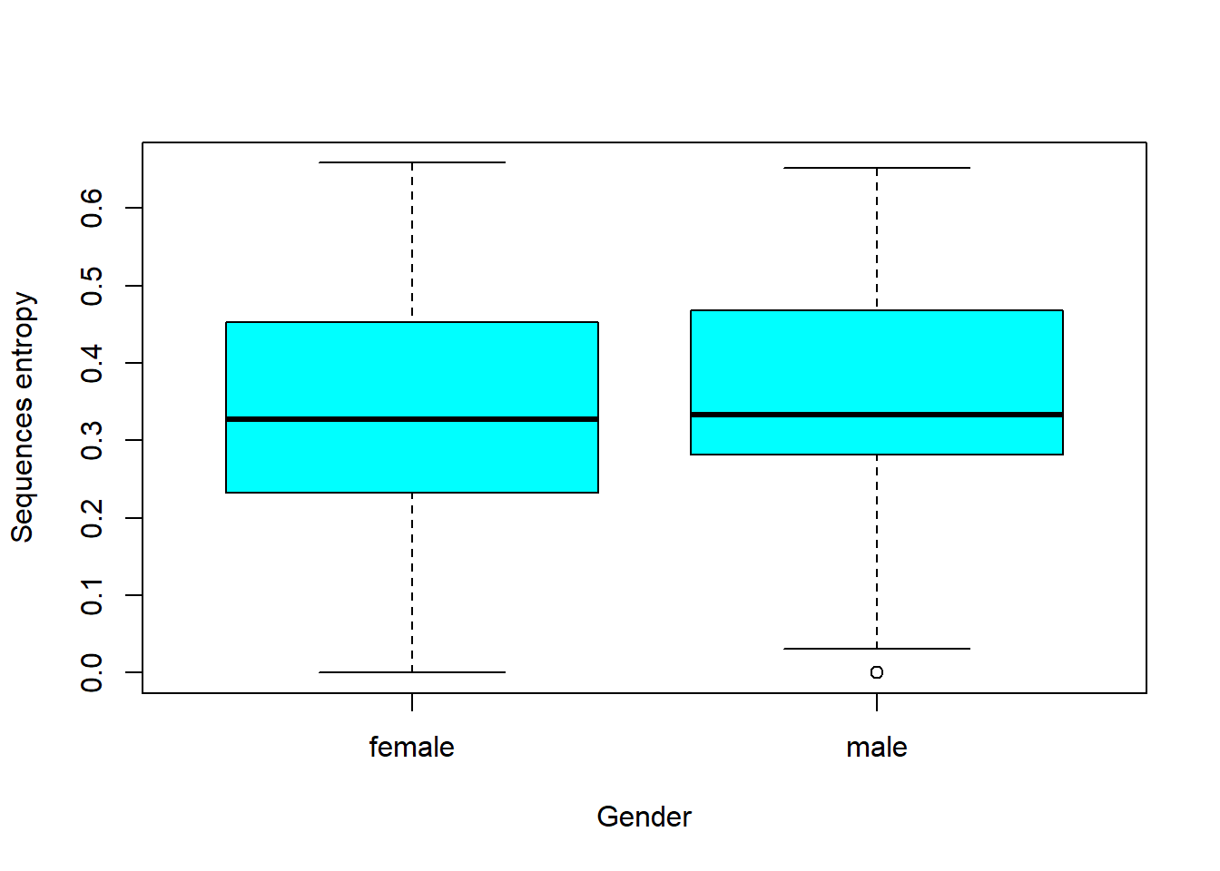
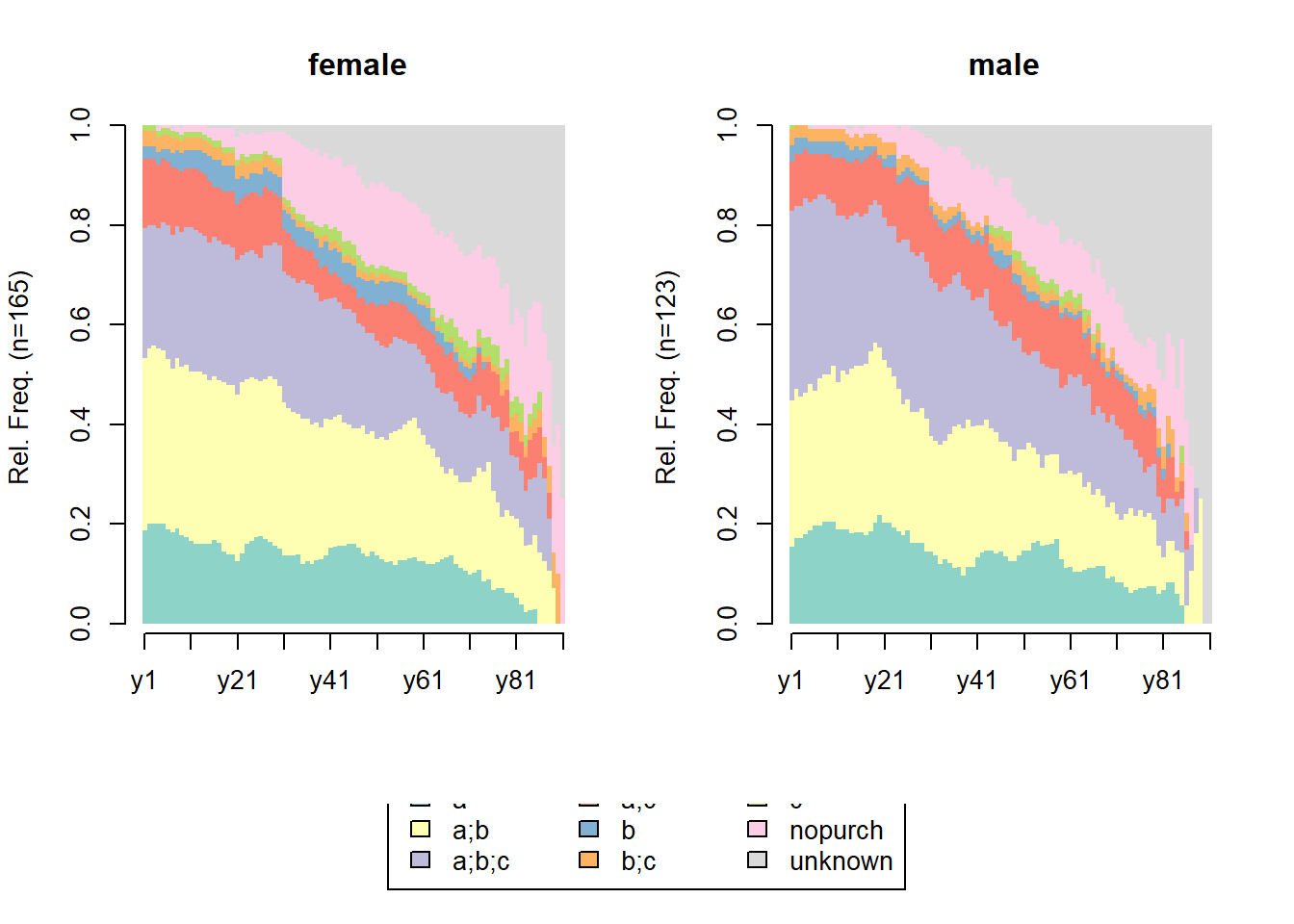
# entrophy distribution based on gender
df.ent <- cbind(df.seq, df.ient)
boxplot(
    Entropy ~ df.feat$sex,
    data = df.ent,
    xlab = 'Gender',
    ylab = 'Sequences entropy',
    col = 'cyan'
)