11 Communication
11.1 Information Theory
11.1.1 Entropy
Most of the examples are taken from philentropy package in R, which can be accessed via this link
11.1.1.1 Discrete Entropy
If \(\mathbf{p}_X = (p_{x1},p_{x2},...,p_{xn})\) is the probability distribution of the discrete random variable X with \(P(X = x) = p_{xi}\). Then, the entropy of the distribution is (Shannon 1948)
\[ H(\mathbf{p}_X) = -\sum_{x_i} p_{xi}\log_2 p_{xi} \]
where
- entropy unit is bits, and \(H(p) \in [0,1]\) and max at \(p = 0.5\)
- or the unit is nats (\(log_e\))
- or the unit is dits (\(log_{10}\))
In general, if you have different bases, you can convert between units. Given bases a and b
\[ \log_a k = \log_a b \times log_b k \]
where \(\log_a b\) is a constant.
Generalize
\[ H_b(X) = log_b a \times H_a(X) \]
Equivalently,
\[ H(X) = E(\frac{1}{\log p(x)}) \]
Entropy is the measure of how much information gained from learning the value of X (Zwillinger 1995, 262). Entropy depends on the distribution of X.
Example:
If X has 2 values, then \(\mathbf{p}= (p,1-p)\) and
\[ H(\mathbf{p}_X ) = H(p,1-p) = -p \log_2 p - (1-p) \log_2 (1-p) \]
which is known as binary entropy function
Plot of p vs. H(p) where max of \(H(\mathbf{p}_X) = \log_2 n\) when \(X \sim U\)
hb <- function(gamma) {
    -gamma * log2(gamma) - (1 - gamma) * log2(1 - gamma) # output in bits
}

xs <- seq(0, 1, len = 100)
plot(xs,
     hb(xs),
     type = 'l',
     xlab = "p",
     ylab = "H(p)")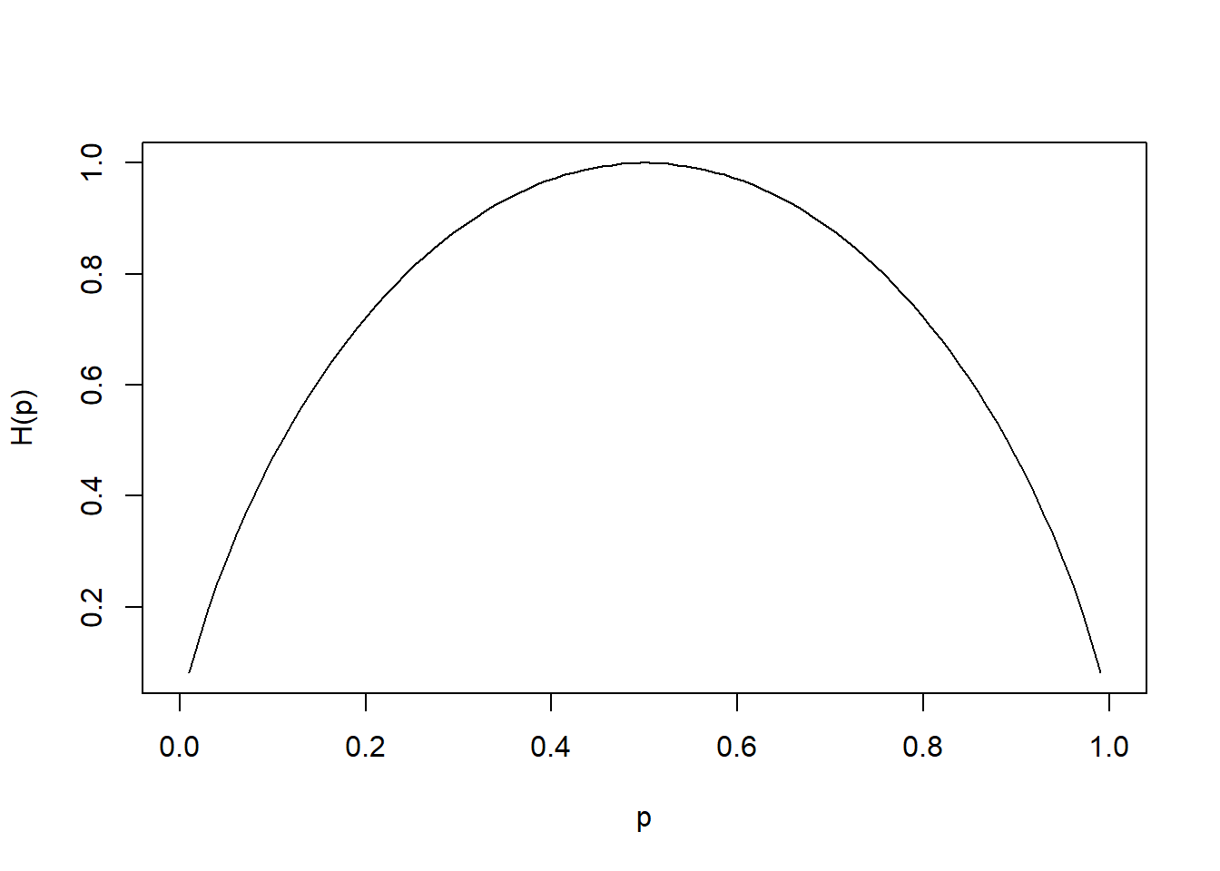
library("philentropy")
Prob <- 1:10/sum(1:10) # probabilities P(X)
H(Prob) # Shannon's Entropy
## [1] 3.10364311.1.1.2 Mutual Information
If X and Y are two discrete random variables and \(\mathbf{p}_{X \times Y}\) is the their joint distribution, the mutual information (i.e., learning of a value of X gives information about the value of Y) of X and Y is
\[ I(X,Y) = I(Y,X) = H(\mathbf{p}_X)+ H(\mathbf{p}_Y)- H(\mathbf{p}_{X \times Y}) \]
where \(I(X,Y) \ge 0\) and \(I(X,Y) = 0\) iff X and Y are independent (information about X gives no information about Y).
Equivalently,
\[ MI(X,Y) = \sum_{i=1}^n \sum_{j=1}^m P(x_i, y_j) \times \log_b (\frac{P(x_i,y_j)}{P(x_i) \times P(y_j)}) \]
Properties:
- \(I(X;X) = H(X)\) known as self-information
- \(I(X;Y) \ge 0\) with equality iff \(X \perp Y\)
P_x <- 1:10/sum(1:10) # distribution P(X)
P_y <- 20:29/sum(20:29) # distribution P(Y)
P_xy <- 1:10/sum(1:10) # joint distribution P(X,Y)
MI(P_x, P_y, P_xy) # Mutual Information
## [1] 3.31197311.1.1.3 Relative Entropy
The measure of the distance between distribution p and q is called relative entropy, denoted by \(D(p ||q)\)
Equivalently, it measures the inefficiency of assuming distribution q when the true distribution is p.
The relative entropy between p(x) and q(x) is
\[ D(p||q) = \sum_x p(x) \log \frac{p(x)}{q(X)} \]
where
- \(D(p||q) \ge 0\) and equality iff \(p = q\)
11.1.1.4 Joint-Entropy
\[ H(X,Y) = - \sum_{i=1}^n \sum_{j = 1}^m P(x_i, y_j) \times \log_b(P(x_i,y_j)) \]
## [1] 3.10364311.1.1.5 Conditional Entropy
\[ H(Y|X) = - \sum_{i=1}^n \sum_{j = 1}^m P(x_i, y_j) \times \log_b(\frac{P(x_i)}{P(x_i,y_j)}) \]
P_x <- 1:10/sum(1:10) # distribution P(X)
P_y <- 1:10/sum(1:10) # distribution P(Y)
CE(P_x, P_y) # Joint-Entropy
## [1] 0Relation among entropy measures
\[ H(X,Y) = H(X) + H(Y|X) = H(Y) + H(X|Y) \]
Properties:
- Chain rule: \(H(X_1, ..., X_n) = \sum_{i=1}^n H(X_i | X_{i-1},...,X_1)\)
- \(0 \le H(Y|X) \le H(Y)\) Information on X does not increase the entropy measure of Y
- If \(X \perp Y\), then \(H(Y|X) = H(Y); H(X,Y) = H(X) + H(Y)\)
- \(H(X) \le log |n_X|\) where \(n_X\) = number of elements in X
- \(H(X) = \log (n_X)\) iff \(X \sim U\)
- \(H(X_1,...,X_n) \le \sum_i^n H(X_i)\)
- \(H(X_1,...,X_n) = \sum_i^n H(X_i)\) iff \(X_i\)’s are mutually independent.
11.1.1.6 Continuous Entropy
If X is a continuous variable, its entropy is
\[ h(\mathbf{X}) = - \int_{R^d} p(\mathbf{x})\log p(\mathbf{x}) dx \]
where d is the dimension of X.
If X and Y are continuous random variables with density functions \(p(\mathbf{x})\) and \(q(\mathbf{y})\), the relative entropy is
\[ H(X,Y) = \int_{R^d} p(x) \log \frac{p(x)}{q(x)} dx \]
More advance analysis can be access here
11.1.2 Divergence
Three metrics for divergence can be found here:
- Kullback-Leibler
- Jensen-Shannon
- Generalized Jensen-Shannon
11.1.3 Channel Capacity
The information channel capacity of a discrete memoryless channel is
\[ C = \max_{p(x)} I(X;Y) \]
which is the highest rate use at which information can be sent without much error.
More information can be found here