13.1 Example
This example is subscription customers by Sergey Bryl’ in which he adapted model Fader and Hardie (2007)
## ── Attaching core tidyverse packages ──────────────────────── tidyverse 2.0.0 ──
## ✔ dplyr     1.1.2     ✔ readr     2.1.4
## ✔ forcats   1.0.0     ✔ stringr   1.5.0
## ✔ ggplot2   3.4.3     ✔ tibble    3.2.1
## ✔ lubridate 1.9.2     ✔ tidyr     1.3.0
## ✔ purrr     1.0.2
## ── Conflicts ────────────────────────────────────────── tidyverse_conflicts() ──
## ✖ dplyr::filter() masks stats::filter()
## ✖ dplyr::lag()    masks stats::lag()
## ℹ Use the conflicted package (<http://conflicted.r-lib.org/>) to force all conflicts to become errors##
## Attaching package: 'reshape2'
##
## The following object is masked from 'package:tidyr':
##
## smiths##
## Attaching package: 'MLmetrics'
##
## The following object is masked from 'package:base':
##
## Recall# retention rate data
df_ret <- data.frame(month_lt = c(0:7),
case01 = c(1, .531, .452, .423, .394, .375, .356, .346),
case02 = c(1, .869, .743, .653, .593, .551, .517, .491),
case03 = c(1, .677, .562, .486, .412, .359, .332, .310),
case04 = c(1, .631, .468, .382, .326, .289, .262, .241)
) %>%
melt(., id.vars = c('month_lt'), variable.name = 'example', value.name = 'retention_rate')
ggplot(df_ret, aes(x = month_lt, y = retention_rate, group = example, color = example)) +
theme_minimal() +
facet_wrap(~ example) +
scale_color_manual(values = c('#4e79a7', '#f28e2b', '#e15759', '#76b7b2')) +
geom_line() +
geom_point() +
theme(plot.title = element_text(size = 20, face = 'bold', vjust = 2, hjust = 0.5),
axis.text.x = element_text(size = 8, hjust = 0.5, vjust = .5, face = 'plain'),
strip.text = element_text(face = 'bold', size = 12)) +
ggtitle('Retention Rate')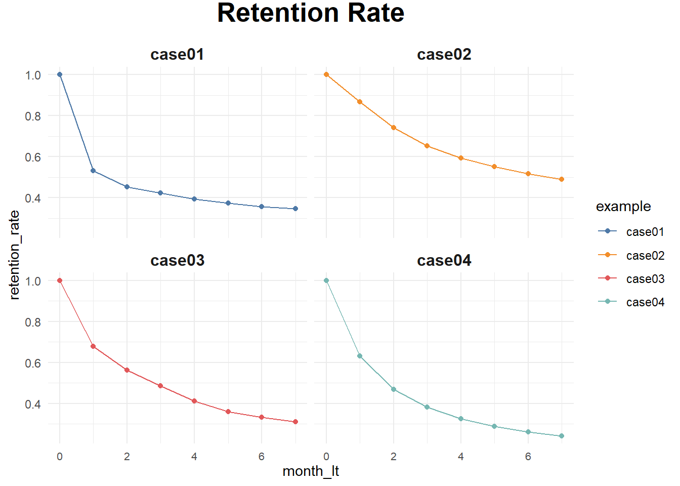
Prediciton when we only have values on certain months
# functions for sBG distribution
churnBG <- Vectorize(function(alpha, beta, period) {
        t1 = alpha / (alpha + beta)
        result = t1
        if (period > 1) {
                result = churnBG(alpha, beta, period - 1) * (beta + period - 2) / (alpha + beta + period - 1)
        }
        return(result)
}, vectorize.args = c("period"))

survivalBG <- Vectorize(function(alpha, beta, period) {
        t1 = 1 - churnBG(alpha, beta, 1)
        result = t1
        if(period > 1){
                result = survivalBG(alpha, beta, period - 1) - churnBG(alpha, beta, period)
        }
        return(result)
}, vectorize.args = c("period"))

MLL <- function(alphabeta) {
        if(length(activeCust) != length(lostCust)) {
                stop("Variables activeCust and lostCust have different lengths: ",
                     length(activeCust), " and ", length(lostCust), ".")
        }
        t = length(activeCust) # number of periods
        alpha = alphabeta[1]
        beta = alphabeta[2]
        return(-as.numeric(
                sum(lostCust * log(churnBG(alpha, beta, 1:t))) +
                        activeCust[t]*log(survivalBG(alpha, beta, t))
        ))
}


df_ret <- df_ret %>%
        group_by(example) %>%
        mutate(activeCust = 1000 * retention_rate,
               lostCust = lag(activeCust) - activeCust,
               lostCust = ifelse(is.na(lostCust), 0, lostCust)) %>%
        ungroup()


ret_preds01 <- vector('list', 7)
for (i in c(1:7)) {

        df_ret_filt <- df_ret %>%
                filter(between(month_lt, 1, i) == TRUE & example == 'case01')

        activeCust <- c(df_ret_filt$activeCust)
        lostCust <- c(df_ret_filt$lostCust)

        opt <- optim(c(1, 1), MLL)
        retention_pred <- round(c(1, survivalBG(alpha = opt$par[1], beta = opt$par[2], c(1:7))), 3)

        df_pred <- data.frame(month_lt = c(0:7),
                              example = 'case01',
                              fact_months = i,
                              retention_pred = retention_pred)
        ret_preds01[[i]] <- df_pred
}
## Warning in log(churnBG(alpha, beta, 1:t)): NaNs produced
## Warning in log(churnBG(alpha, beta, 1:t)): NaNs produced## Warning in log(survivalBG(alpha, beta, t)): NaNs produced## Warning in log(churnBG(alpha, beta, 1:t)): NaNs produced## Warning in log(survivalBG(alpha, beta, t)): NaNs produced## Warning in log(churnBG(alpha, beta, 1:t)): NaNs produced## Warning in log(survivalBG(alpha, beta, t)): NaNs produced## Warning in log(churnBG(alpha, beta, 1:t)): NaNs produced## Warning in log(survivalBG(alpha, beta, t)): NaNs producedret_preds01 <- as.data.frame(do.call('rbind', ret_preds01))
ret_preds02 <- vector('list', 7)
for (i in c(1:7)) {
df_ret_filt <- df_ret %>%
filter(between(month_lt, 1, i) == TRUE & example == 'case02')
activeCust <- c(df_ret_filt$activeCust)
lostCust <- c(df_ret_filt$lostCust)
opt <- optim(c(1, 1), MLL)
retention_pred <- round(c(1, survivalBG(alpha = opt$par[1], beta = opt$par[2], c(1:7))), 3)
df_pred <- data.frame(month_lt = c(0:7),
example = 'case02',
fact_months = i,
retention_pred = retention_pred)
ret_preds02[[i]] <- df_pred
}## Warning in log(churnBG(alpha, beta, 1:t)): NaNs produced## Warning in log(churnBG(alpha, beta, 1:t)): NaNs produced
## Warning in log(churnBG(alpha, beta, 1:t)): NaNs produced

## Warning in log(churnBG(alpha, beta, 1:t)): NaNs produced
## Warning in log(churnBG(alpha, beta, 1:t)): NaNs produced
## Warning in log(churnBG(alpha, beta, 1:t)): NaNs produced
## Warning in log(churnBG(alpha, beta, 1:t)): NaNs producedret_preds02 <- as.data.frame(do.call('rbind', ret_preds02))
ret_preds03 <- vector('list', 7)
for (i in c(1:7)) {
df_ret_filt <- df_ret %>%
filter(between(month_lt, 1, i) == TRUE & example == 'case03')
activeCust <- c(df_ret_filt$activeCust)
lostCust <- c(df_ret_filt$lostCust)
opt <- optim(c(1, 1), MLL)
retention_pred <- round(c(1, survivalBG(alpha = opt$par[1], beta = opt$par[2], c(1:7))), 3)
df_pred <- data.frame(month_lt = c(0:7),
example = 'case03',
fact_months = i,
retention_pred = retention_pred)
ret_preds03[[i]] <- df_pred
}
ret_preds03 <- as.data.frame(do.call('rbind', ret_preds03))
ret_preds04 <- vector('list', 7)
for (i in c(1:7)) {
df_ret_filt <- df_ret %>%
filter(between(month_lt, 1, i) == TRUE & example == 'case04')
activeCust <- c(df_ret_filt$activeCust)
lostCust <- c(df_ret_filt$lostCust)
opt <- optim(c(1, 1), MLL)
retention_pred <- round(c(1, survivalBG(alpha = opt$par[1], beta = opt$par[2], c(1:7))), 3)
df_pred <- data.frame(month_lt = c(0:7),
example = 'case04',
fact_months = i,
retention_pred = retention_pred)
ret_preds04[[i]] <- df_pred
}
ret_preds04 <- as.data.frame(do.call('rbind', ret_preds04))
ret_preds <- bind_rows(ret_preds01, ret_preds02, ret_preds03, ret_preds04)
df_ret_all <- df_ret %>%
select(month_lt, example, retention_rate) %>%
left_join(., ret_preds, by = c('month_lt', 'example'))
ggplot(df_ret_all, aes(x = month_lt, y = retention_rate, group = example, color = example)) +
theme_minimal() +
facet_wrap(~ example) +
scale_color_manual(values = c('#4e79a7', '#f28e2b', '#e15759', '#76b7b2')) +
geom_line(size = 1.5) +
geom_point(size = 1.5) +
geom_line(aes(y = retention_pred, group = fact_months), alpha = 0.5) +
theme(plot.title = element_text(size = 20, face = 'bold', vjust = 2, hjust = 0.5),
axis.text.x = element_text(size = 8, hjust = 0.5, vjust = .5, face = 'plain'),
strip.text = element_text(face = 'bold', size = 12)) +
ggtitle('Retention Rate Projections')## Warning: Using `size` aesthetic for lines was deprecated in ggplot2 3.4.0.
## ℹ Please use `linewidth` instead.
## This warning is displayed once every 8 hours.
## Call `lifecycle::last_lifecycle_warnings()` to see where this warning was
## generated.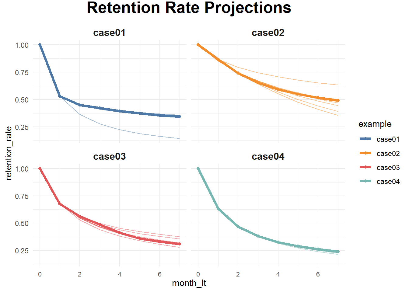
calculate the average LTV for case03 based on two historical months with a forecast horizon of 24 months and a subscription price of $1
### LTV prediction ###
df_ltv_03 <- df_ret %>%
        filter(between(month_lt, 1, 2) == TRUE & example == 'case03')

activeCust <- c(df_ltv_03$activeCust)
lostCust <- c(df_ltv_03$lostCust)

opt <- optim(c(1, 1), MLL)
retention_pred <- round(c(survivalBG(alpha = opt$par[1], beta = opt$par[2], c(3:24))), 3)

df_pred <- data.frame(month_lt = c(3:24),
                      retention_pred = retention_pred)

df_ltv_03 <- df_ret %>%
        filter(between(month_lt, 0, 2) == TRUE & example == 'case03') %>%
        select(month_lt, retention_rate) %>%
        bind_rows(., df_pred) %>%
        mutate(retention_rate_calc = ifelse(is.na(retention_rate), retention_pred, retention_rate),
               ltv_monthly = retention_rate_calc * 1,
               ltv_cum = round(cumsum(ltv_monthly), 2))
# average LTV of $9.33. actual data for the observed periods (from 0 to 2nd months) and the predicted retention for the future periods (from 3rd to 24th months)