21.6 Market Response Model
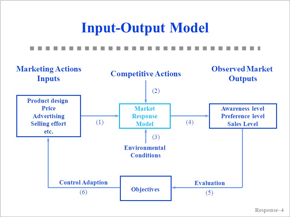
Marketing Inputs:
- Selling effort
- advertising spending
- promotional spending
Marketing Outputs:
- sales
- share
- profit
- awareness
Give phenomena for a good model:
- P1: Dynamic sales response involves a sales growth rate and a sales decay rate that are different
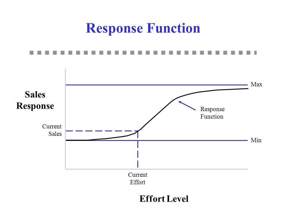
- P2: Steady-state response can be concave or S-shaped. Positive sales at 0 adverting.
- P3: Competitive effects
- P4: Advertising effectiveness dynamics due to changes in media, copy, and other factors.
- P5: Sales still increase or fall off even as advertising is held constant.
Saunder (1987) phenomena
- P1: Output = 0 when Input = 0
- P2: The relationship between input and output is linear
- P3: Returns decrease as the scale of input increases (i.e., additional unit of input gives less output)
- P4: Output cannot exceed some level (i.e., saturation)
- P5: Returns increase as scale of input increases (i.e., additional unit of input gives more output)
- P6: Returns first increase and then decrease as input increases (i.e., S-shaped return)
- P7: Input must exceed some level before it produces any output (i.e., threshold)
- P8: Beyond some level of input, output declines (i.e., supersaturation point)
Aggregate Response Models
Linear model: \(Y = a + bX\)
Through origin
can only handle constant returns to scale (i.e., can’t handle concave, convex, and S-shape)
The Power Series/Polynomial model: \(Y = a + bX + c X^2 + dX^3 + ...\)
- can’t handle saturation and threshold
Fraction root model/ Power model: \(Y = a+bX^c\) where c is prespecified
c = 1/2, called square root model
c = -1, called reciprocal model
c can be interpreted as elasticity if a = 0.
c = 1, linear
c <1, decreasing return
c>1, increasing returns
Semilog model: \(Y = a + b \ln X\)
- Good when constant percentage increase in marketing effort (X) result in constant absolute increase in sales (Y)
Exponential model: \(Y = ae^{bX}\) where X >0
b > 0, increasing returns and convex
b < 0, decreasing returns and saturation
Modified exponential model: \(Y = a(1-e^{-bX}) +c\)
Decreasing returns and saturation
upper bound = a + c
lower bound = c
typically used in selling effort
Logistic model: \(Y = \frac{a}{a+ e^{-(b+cX)}}+d\)
increasing return followed by decreasing return to scale, S-shape
saturation = a + d
good with saturation and s-shape
Gompertz model
ADBUDG model (Little 1970) : \(Y = b + (a-b)\frac{X^c}{d + X^c}\)
c > 1, S-shaped
0 < c < 1
Concave
saturation effect
upper bound at a
lower bound at b
typically used in advertising and selling effort.
can handle, through origin, concave, saturation, S-shape
Additive model for handling multiple Instruments: \(Y = af(X_1) + bg(X_2)\)
Multiplicative model for handling multiple instruments: \(Y = aX_1^b X_2^c\) where c and c are elasticities. More generally, \(Y = af(X_1)\times bg(X_2)\)
Multiplicative and additive model: \(Y = af(X_1) + bg(X_2) + cf(X_1) g(X_2)\)
Dynamic response model: \(Y_t = a_0 + a_1 X_t + \lambda Y_{t-1}\) where \(a_1\) = current effect, \(\lambda\) = carry-over effect
Dynamic Effects
Carry-over effect: current marketing expenditure influences future sales
- Advertising adstock/ advertising carry-over is the same thing: lagged effect of advertising on sales
Delayed-response effect: delays between when marketing investments and their impact
Customer holdout effects
Hysteresis effect
New trier and wear-out effect
Stocking effect
Simple Decay-effect model:
\[ A_t = T_t + \lambda T_{t-1}, t = 1,..., \]
where
- \(A_t\) = Adstock at time t
- \(T_t\) = value of advertising spending at time t
- \(\lambda\) = decay/ lag weight parameter
Response Models can be characterized by:
The number of marketing variables
whether they include competition or not
the nature of the relationship between the input variables
- Linear vs. S-shape
whether the situation is static vs. dynamic
whether the models reflect individual or aggregate response
the level of demand analyzed
- sales vs. market share
Market Share Model and Competitive Effects: \(Y = M \times V\) where
Y = Brand sales models
V = product class sales models
M = market-share models
Market share (attraction) models
\[ M_i = \frac{A_i}{A_1 + ..+ A_n} \]
where \(A_i\) attractiveness of brand i
Individual Response Model:
Multinomial logit model representing the probability of individual i choosing brand l is
\[ P_{il} = \frac{e^{A_{il}}}{\sum_j e^{A_{ij}}} \]
where
- \(A_{ij}\) = attractiveness of product j for individual i \(A_{ij} = \sum_k w_k b_{ijk}\)
- \(b_{ijk}\) = individual i’s evaluation of product j on product attribute k, where the summation is over all the products that individual
iis considering to purchase - \(w_k\) = importance weight associated with attribute k in forming product preferences.

