4.1 Simulating equally likely outcomes

Consider again two rolls of a fair four-sided and let $X$ be the sum and $Y$ the larger of the two rolls (or the common value if a tie). In the previous chapter we used a box model to specify the probability space correspoding to pairs of rolls of a four-sided die. When tickets are equally likely and sampled with replacement, a Discrete Uniform model can also be used. Think of a DiscreteUniform(a, b) probability space corresponding to a spinner with sectors of equal area labeled with integer values from a to b (inclusive). For example, the spinner in Figure 3.2 corresponds to DiscreteUniform(1, 4).

In the following, $U$ represents the result of a single roll of a fair four-sided die. The default mapping function in RV is the identity, so U = RV(P) represents⁷¹ $U(\omega) = \omega$.

P = DiscreteUniform(a = 1, b = 4)
U = RV(P)

U.sim(10000).plot()
plt.show()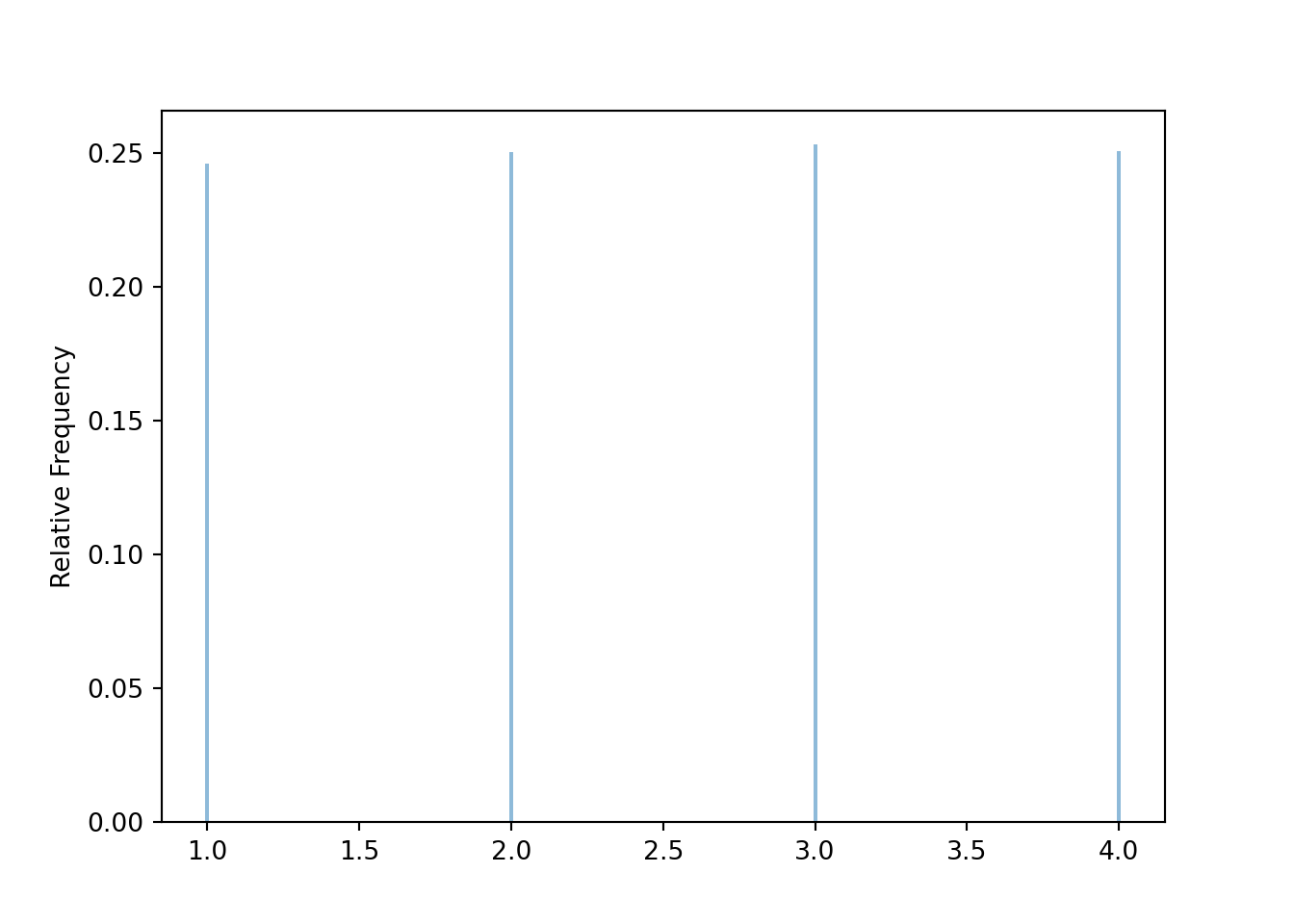

For two rolls the probability space corresponds to spinning the DiscreteUniform spinner twice, which is coded⁷² as DiscreteUniform(a = 1, b = 4) ** 2. The first line below has the same effect⁷³ as BoxModel([1, 2, 3, 4], size = 2, replace = True).

P = DiscreteUniform(a = 1, b = 4) ** 2
X = RV(P, sum)
Y = RV(P, max)

(X & Y).sim(10000).plot(['tile', 'marginal'])
plt.show()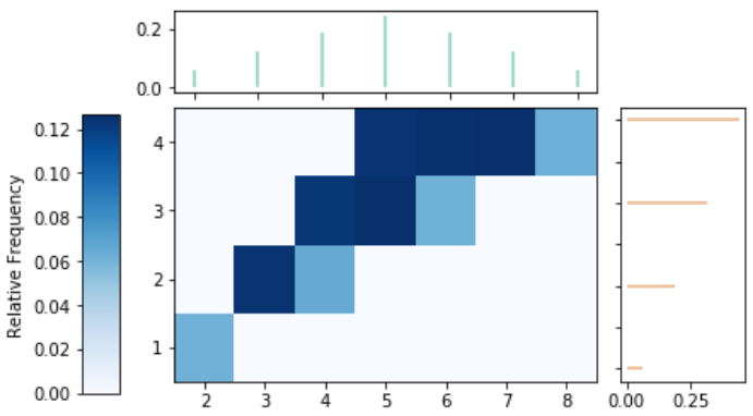

$Tile and impulse plot visualization of the simulation-based approximate joint and marginal distributions of the sum ($X$) and larger ($Y$) of two rolls of a fair four-sided die.$

Figure 4.1: Tile and impulse plot visualization of the simulation-based approximate joint and marginal distributions of the sum ($X$) and larger ($Y$) of two rolls of a fair four-sided die.

For technical reasons, Symbulate will not plot simulated outcomes from a ProbabilitySpace, only simulated realizations of an RV. Essentially, as mentioned in earlier sections, probability space outcomes can be anything — not necessarily numbers — and so there are too many potential situations and plots for Symbulate to handle with a single plot command. In contrast, simulated realizations of RV are numbers (or vectors of numbers) which facilitates plotting. Plotting simulated outcomes from a probability space P with numerical outcomes can be achieved by first defining X = RV(P) and then simulating and plotting values of X. That is, replace P.sim(10000).plot() with RV(P).sim(10000).plot(). However, this only works if the outcomes of P are numerical.↩︎
For now you can interpretDiscreteUniform(a = 1, b = 4) as a spinner with four quarters labeled 1, 2, 3, 4, and ** 2 as “spin the spinner twice”. In Python, ** represents exponentiation; e.g., 2 ** 5 = 32. So DiscreteUniform(a = 1, b = 4) ** 2 is equivalent to DiscreteUniform(a = 1, b = 4) * DiscreteUniform(a = 1, b = 4). Future sections will reveal why the product * notation is natural for independent spins of spinners.↩︎
BoxModel assumes equally likely tickets by default, but there are options for non-equally likely cases.↩︎