2.6 Relative frequencies

A simulation involves repeatedly artificially recreating the random phenomenon a large number of times and using the results to investigate properties of interest. In particular, we can use simulation-based relative frequencies to approximate probabilities. That is, the probability of event \(A\) can be approximated by simulating, according to the assumptions corresponding to the probability measure \(\textrm{P}\), the random phenomenon a large number of times and computing the relative frequency of \(A\).

\[ {\small \textrm{P}(A) \approx \frac{\text{number of repetitions on which $A$ occurs}}{\text{number of repetitions}}, \quad \text{for a large number of repetitions simulated according to $\textrm{P}$} } \]

In practice, many repetitions of a simulation are performed on a computer to approximate what happens in the “long run”. However, we often start by carrying out a few repetitions by hand to help make the process more concrete.

Example 2.29 Use a four-sided die (or a box or a spinner) and perform by hand 10 repetitions of the simulation in Example 2.26. (Yes, really do it.) For each repetition, record the results of the first and second rolls (or draws or spins) and the values of \(X\) and \(Y\). Based only on the results of your simulation, how would you approximate the following? (Don’t worry if the approximations are any good yet.)

1. \(\textrm{P}(A)\), where \(A\) is the event that the first roll is 3.
2. \(\textrm{P}(X=6)\)
3. \(\textrm{P}(X \ge 6)\)
4. \(\textrm{P}(Y = 3)\)
5. \(\textrm{P}(Y \ge 3)\)
6. \(\textrm{P}(X=6, Y=3)\)
7. \(\textrm{P}(X\ge6, Y \ge 3)\)

Solution. to Example 2.29.

Show/hide solution

See Table 2.19 for the results of our simulation.

1. Approximate \(\textrm{P}(A)\) by 4/10, the relative frequency of event \(A\) in the simulation; that is, the proportion of repetitions where the first roll is 3.
2. Approximate \(\textrm{P}(X=6)\) by 2/10, the proportion of repetitions where the sum is 6.
3. Approximate \(\textrm{P}(X\ge 6)\) by 5/10, the proportion of repetitions where the sum is at least 6.
4. Approximate \(\textrm{P}(Y=3)\) by 3/10, the proportion of repetitions where the max is 3.
5. Approximate \(\textrm{P}(Y\ge 3)\) by 7/10, the proportion of repetitions where the max is at least 3.
6. Approximate \(\textrm{P}(X=6, Y = 3)\) by 1/10, the proportion of repetitions where both the sum is 6 and the max is 3.
7. Approximate \(\textrm{P}(X\ge 6, Y \ge 3)\) by 5/10, the proportion of repetitions where both the sum is at least 6 and the max is at least 3. (Since \(X\ge 6\) implies \(Y\ge 3\), \(\textrm{P}(X\ge 6, Y\ge 3) = \textrm{P}(X\ge 6)\).)

Table 2.19 summarizes the results of 10 repetitions of the simulation in Example 2.29. Results vary naturally so your simulation results will be different, but the same ideas apply.

Table 2.19: Results of 10 repetitions of two rolls of a fair four-sided die. X is the sum of the two rolls, Y is the maximum, and A is the event that the first roll is a 3.

Repetition	First roll	Second roll	X	Y	Event A occurs?	I[A]
1	2	1	3	2	False	0
2	1	1	2	1	False	0
3	3	3	6	3	True	1
4	4	3	7	4	False	0
5	3	2	5	3	True	1
6	3	4	7	4	True	1
7	2	3	5	3	False	0
8	2	4	6	4	False	0
9	1	2	3	2	False	0
10	3	4	7	4	True	1

Remember that it is important to distinguish between what entails (1) one repetition of the simulation and its output, and (2) the simulation itself and output from many repetitions. When describing a simulation, refrain from making vague statements like “repeat this” or “do it again”, because “this” or “it” could refer to different elements of the simulation. In the dice example, (1) rolling a die is repeated to generate a single \((X, Y)\) pair, and (2) the process of generating \((X, Y)\) pairs is repeated to obtain the simulation⁵² results. That is, a single repetition involves an ordered pair of die rolls, resulting in an outcome \(\omega\), and the values of the sum \(X(\omega)\) and max \(Y(\omega)\) are computed for the outcome \(\omega\). The process described in the previous sentence is repeated many times to generate many outcomes and \((X, Y)\) pairs according to the probability model.

Think of simulation results being organized in a table like Table 2.19, where each row corresponds to a different repetition of the simulation and each column corresponds to a different random variable or event. Remember that indicators are the bridge between events and random variables. On each repetition of the simulation an event either occurs or not. We could record the occurrence of an event as “True/False” for each repetition, or we could record the 1/0 value of the corresponding indicator random variable; see the last two columns in Table 2.19 for an example.

Example 2.30 Continuing Example 2.29.

1. Construct a table of the simulated relative frequencies of each possible value \(x\) of \(X\).
2. Construct a table of the simulated relative frequencies of each possible value \((x, y)\) pair of \((X, y)\).

Solution. to Example 2.30.

Show/hide solution

For discrete random variables like these we can make tables or plots summarizing the observed values of the random variables and their corresponding relative frequencies.

Summarizing our simulation results from Table 2.19, the observed values of \(X\) and corresponding relative frequencies are

\(x\)	Relative frequency
2	1/10
3	2/10
4	0
5	2/10
6	2/10
7	3/10
8	0

The above table⁵³ represents an approximation of the distribution of \(X\) (albeit a bad approximation); compare with Table 2.11.

We can summarize simulated \((X, Y)\) pairs and their relative frequencies, as in the following two-way table (compare with Table 2.14.

\(x, y\)	1	2	3	4
2	1/10	0	0	0
3	0	2/10	0	0
4	0	0	0	0
5	0	0	2/10	0
6	0	0	1/10	1/10
7	0	0	0	3/10
8	0	0	0	0

Simulation results are summarized in tables and plots. Figure 2.15 displays two plots summarizing the results in Table 2.19. Each dot represents the results of one repetition; the plot on the left displays the simulated \((X, Y)\) pairs, and the plot on the right displays the simulated values of \(X\) alone along with their frequencies. While this simulation only consists of 10 repetitions, a larger scale simulation and the summarization of results would follow the same process.

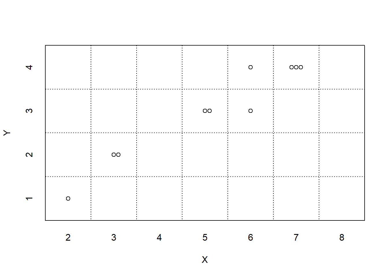
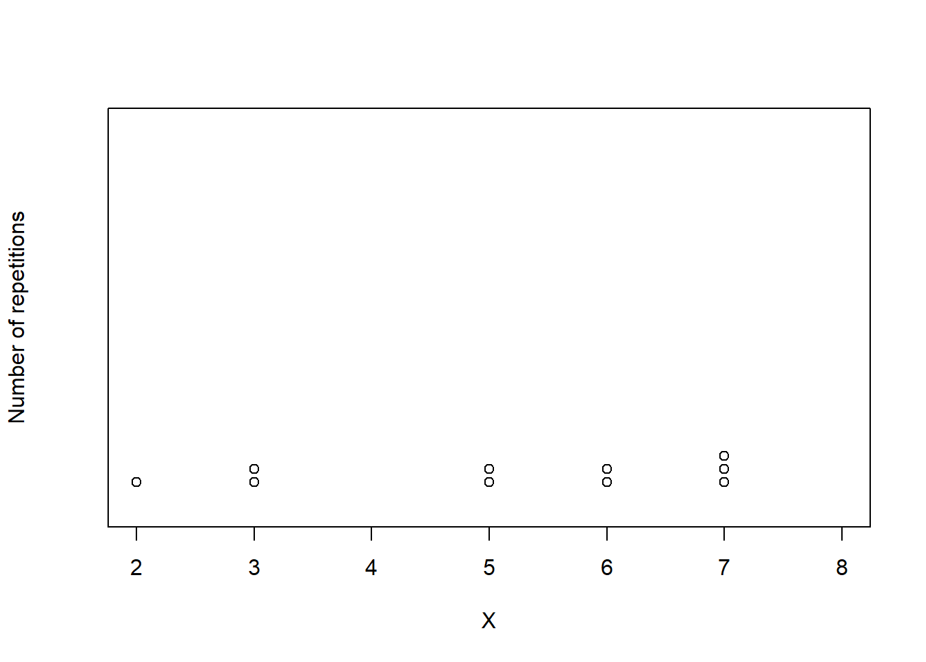
Figure 2.15: Plot summaries of the simulation results in Table 2.19 of 10 repetitions of two rolls of a fair four-sided die, where \(X\) is the sum and \(Y\) is the larger (or common value if a tie) of the two rolls.

You might have noticed that many of the simulated relative frequencies in Example 2.29 provide terrible estimates of the corresponding probabilities. For example, the true probability that the first roll is a 3 is \(\textrm{P}(A) = 0.25\) while the simulated relative frequency is 0.4. The problem is that the simulation only consisted of 10 repetitions. Probabilities can be approximated by long run relatively frequencies, but 10 repetitions certainly doesn’t qualify as the long run! The more repetitions we perform the better our estimates should be. But how many repetitions is sufficient? And how accurate are the estimates? We will address these issues in Section 2.6.2.

2.6.1 A few Symbulate commands for summarizing simulation output

We’ll continue with the dice rolling example. Recall the setup.

P = DiscreteUniform(1, 4) ** 2

X = RV(P, sum)

Y = RV(P, max)

First we’ll simulate and store 10 values of \(X\).

x = X.sim(10)
x # displays the simulated values

Index	Result
0	3
1	5
2	7
3	3
4	5
5	6
6	2
7	4
8	6
...	...
9	7

Suppose we want to find the relative frequency of 6. We can count the number of simulated values equal to 6 with count_eq().

x.count_eq(6)

## 2

The count is the frequency. To find the relative frequency we simply divide by the number of simulated values.

x.count_eq(6) / 10

## 0.2

We can find frequencies of other events using the “count” functions:

• count_eq(u): count equal to u
• count_neq(u): count not equal to u
• count_leq(u): count less than or equal to u
• count_lt(u): count less than u
• count_geq(u): count greater than or equal to u
• count_gt(u): count greater than u
• count: count according to a specified True/False criteria.

Using count() with no inputs to defaults to “count all”, which provides a way to count the total number of simulated values. (This is especially useful when conditioning.)

x.count_eq(6) / x.count()

## 0.2

The tabulate method provides a quick summary of the individual simulated values and their frequencies.

x.tabulate()

Value	Frequency
2	1
3	2
4	1
5	2
6	2
7	2
Total	10

By default, tabulate returns frequencies (counts). Adding the argument⁵⁴ normalize = True returns relative frequencies (proportions).

x.tabulate(normalize = True)

Value	Relative Frequency
2	0.1
3	0.2
4	0.1
5	0.2
6	0.2
7	0.2
Total	1.0

We often initially simulate a small number of repetitions to see what the simulation is doing and check that it is working properly. However, in order to accurately approximate probabilities or distribution we simulate a large number of repetitions (usually thousands for our purposes). Now let’s simulate many \(X\) values and summarize the results.

x = X.sim(10000)

x.tabulate(normalize = True)

Value	Relative Frequency
2	0.0609
3	0.1208
4	0.1935
5	0.2485
6	0.1889
7	0.1287
8	0.0587
Total	1.0

Compare the simulation results to the theoretical probabilities in Table 2.11.

Graphical summaries play an important role in analyzing simulation output. We have previously seen rug plots of individual simulated values. Rug plot emphasize that realizations of a random variable are numbers along a number line. However, a rug plot does not adequately summarize relative frequencies. Instead, calling .plot() produces⁵⁵ an impulse plot which displays the simulated values and their relative frequencies; see Figure 2.16. Since the simulated values are stored as x, the same simulated values are used to produce the table and the plot.

x.plot()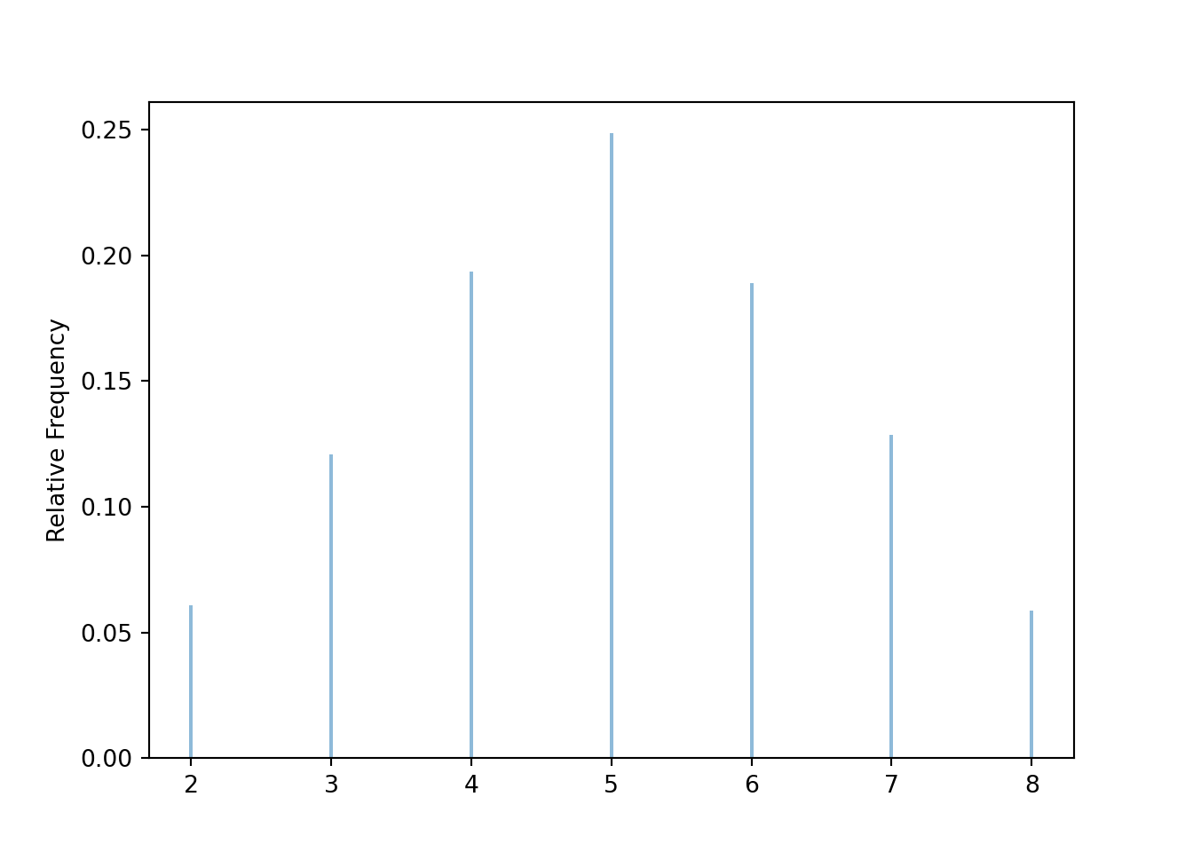

Figure 2.16: Simulation-based approximate distribution of \(X\), the sum of two rolls of a fair four-sided die.

We will introduce several more plot types and commands for summarizing simulation output in following sections.

Figure 2.17 contains a summary of a simulated \(Y\) values. Compare with Table 2.12.

y = Y.sim(10000)
y.tabulate()

Value	Frequency
1	598
2	1875
3	3068
4	4459
Total	10000

y.plot()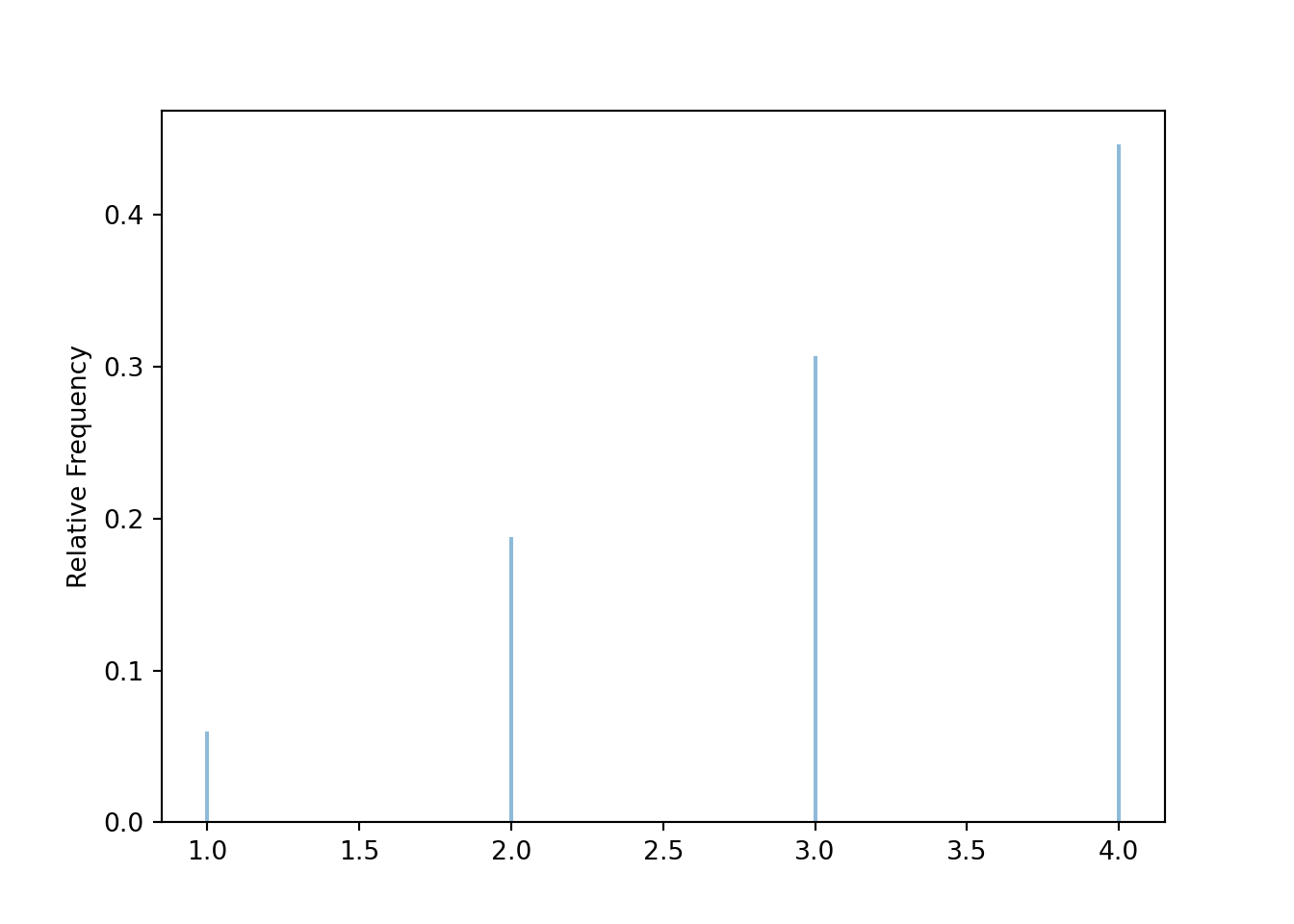

Figure 2.17: Simulation-based approximate distribution of \(Y\), the larger (or common value if a tie) of two rolls of a fair four-sided die.

Now we simulate and summarize a few \((X, Y)\) pairs.

x_and_y = (X & Y).sim(10)
x_and_y 

Index	Result
0	(5, 4)
1	(4, 2)
2	(5, 3)
3	(5, 4)
4	(4, 3)
5	(5, 4)
6	(4, 2)
7	(5, 4)
8	(7, 4)
...	...
9	(5, 3)

Pairs of values can also be tabulated.

x_and_y.tabulate()

Value	Frequency
(4, 2)	2
(4, 3)	1
(5, 3)	2
(5, 4)	4
(7, 4)	1
Total	10

x_and_y.tabulate(normalize = True)

Value	Relative Frequency
(4, 2)	0.2
(4, 3)	0.1
(5, 3)	0.2
(5, 4)	0.4
(7, 4)	0.1
Total	1.0

Individual pairs can be plotted in a scatter plot, which is a two-dimensional analog of a rug plot.

x_and_y.plot()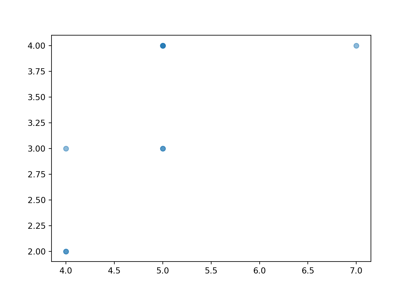

The values can be “jittered” slightly, as below, so that points do not coincide.

x_and_y.plot(jitter = True)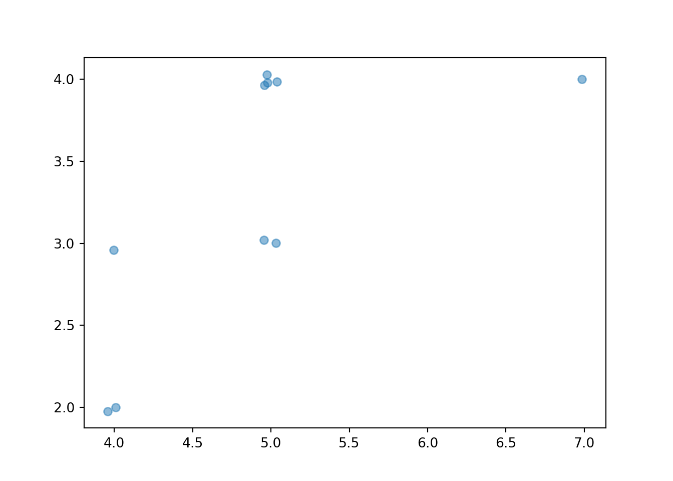

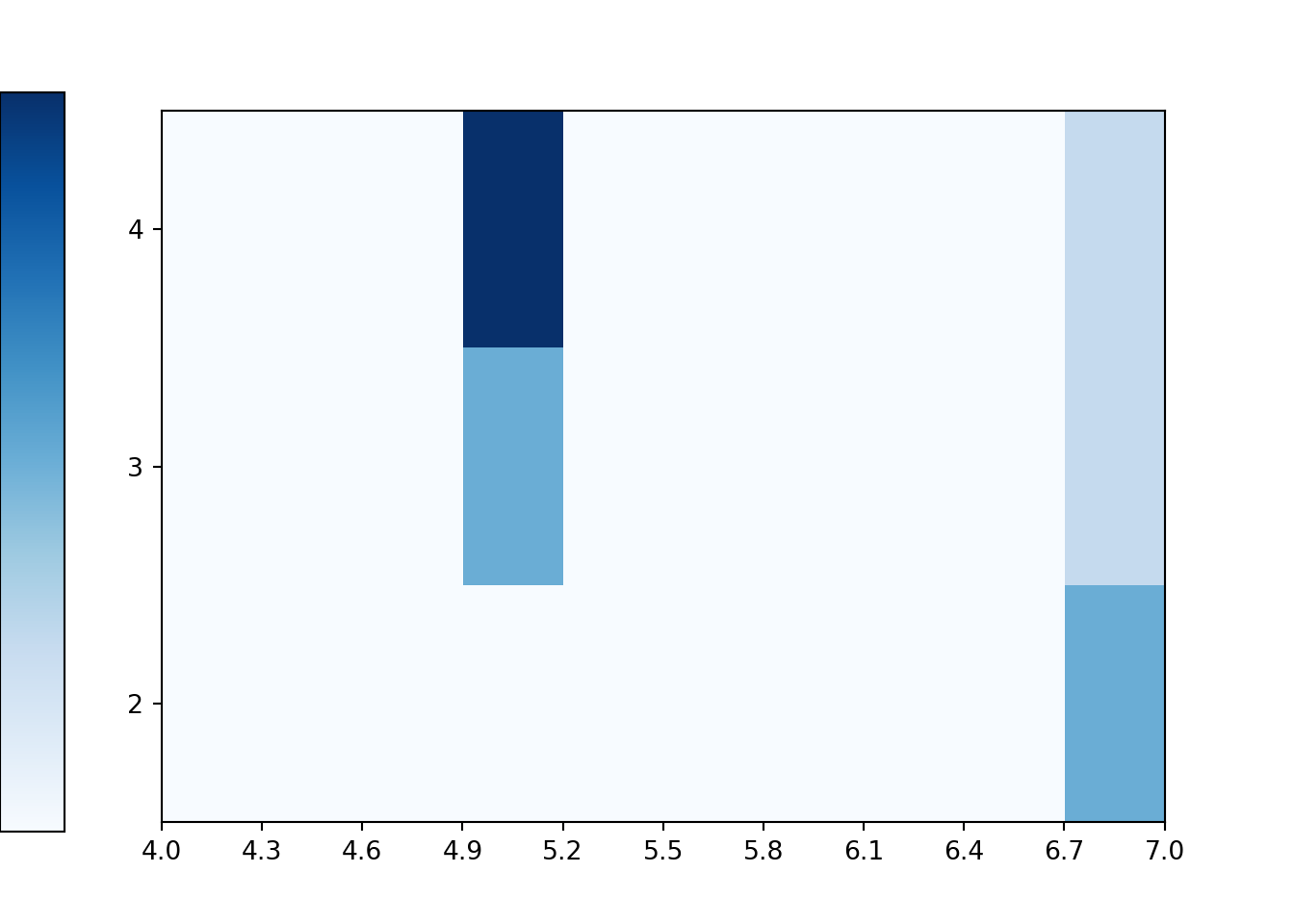
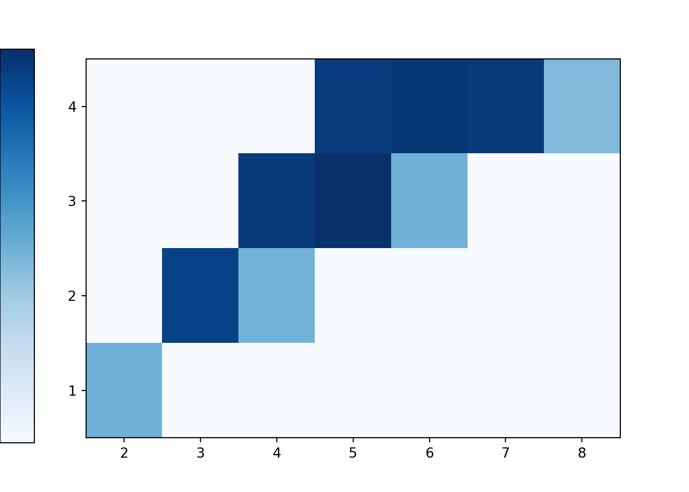
The two-dimensional analog of an impulse plot is a tile plot. For two discrete variables, the 'tile' plot type produces a tile plot (a.k.a. heat map) where rectangles represent the simulated pairs with their relative frequencies visualized on a color scale.

x_and_y.plot('tile')

Custom functions can be used with count to compute relative frequencies of events involving multiple random variables. Suppose we want to approximate \(\textrm{P}(X<6, Y \ge 2)\). We first define a Python function which takes as an input a pair u = (u[0], u[1]) and returns True if u[0] < 6 and u[1] >= 2.

def is_x_lt_6_and_y_ge_2(u):
  if u[0] < 6 and u[1] >= 2:
    return True
  else:
    return False

Now we can use this function along with count to find the simulated relative frequency of the event \(\{X <6, Y \ge 2\}\). Remember that x_and_y stores \((X, Y)\) pairs of values, so the first coordinate x_and_y[0] represents values of \(X\) and the second coordinate x_and_y[1] represents values of \(Y\).

x_and_y.count(is_x_lt_6_and_y_ge_2) / x_and_y.count()

## 0.9

We could also count use Boolean logic; basically using indicators and the property \(\textrm{I}_{\{X<6,Y\ge 2\}}=\textrm{I}_{\{X<6\}}\textrm{I}_{\{Y\ge 2\}}\).

((x_and_y[0] < 6) * (x_and_y[1] >= 2)).count_eq(True) / x_and_y.count()

## 0.9

Now we simulate and many \((X, Y)\) pairs and summarize their frequencies.

x_and_y = (X & Y).sim(10000)

x_and_y.tabulate()

Value	Frequency
(2, 1)	633
(3, 2)	1210
(4, 2)	625
(4, 3)	1251
(5, 3)	1306
(5, 4)	1240
(6, 3)	628
(6, 4)	1269
(7, 4)	1252
(8, 4)	586
Total	10000

Here are the relative frequencies; compare with Table 2.13.

x_and_y.tabulate(normalize = True)

Value	Relative Frequency
(2, 1)	0.0633
(3, 2)	0.121
(4, 2)	0.0625
(4, 3)	0.1251
(5, 3)	0.1306
(5, 4)	0.124
(6, 3)	0.0628
(6, 4)	0.1269
(7, 4)	0.1252
(8, 4)	0.0586
Total	0.9999999999999999

When there are thousands of simulated pairs, a scatter plot does not adequately display relative frequencies, even with jittering.

x_and_y.plot(jitter = True)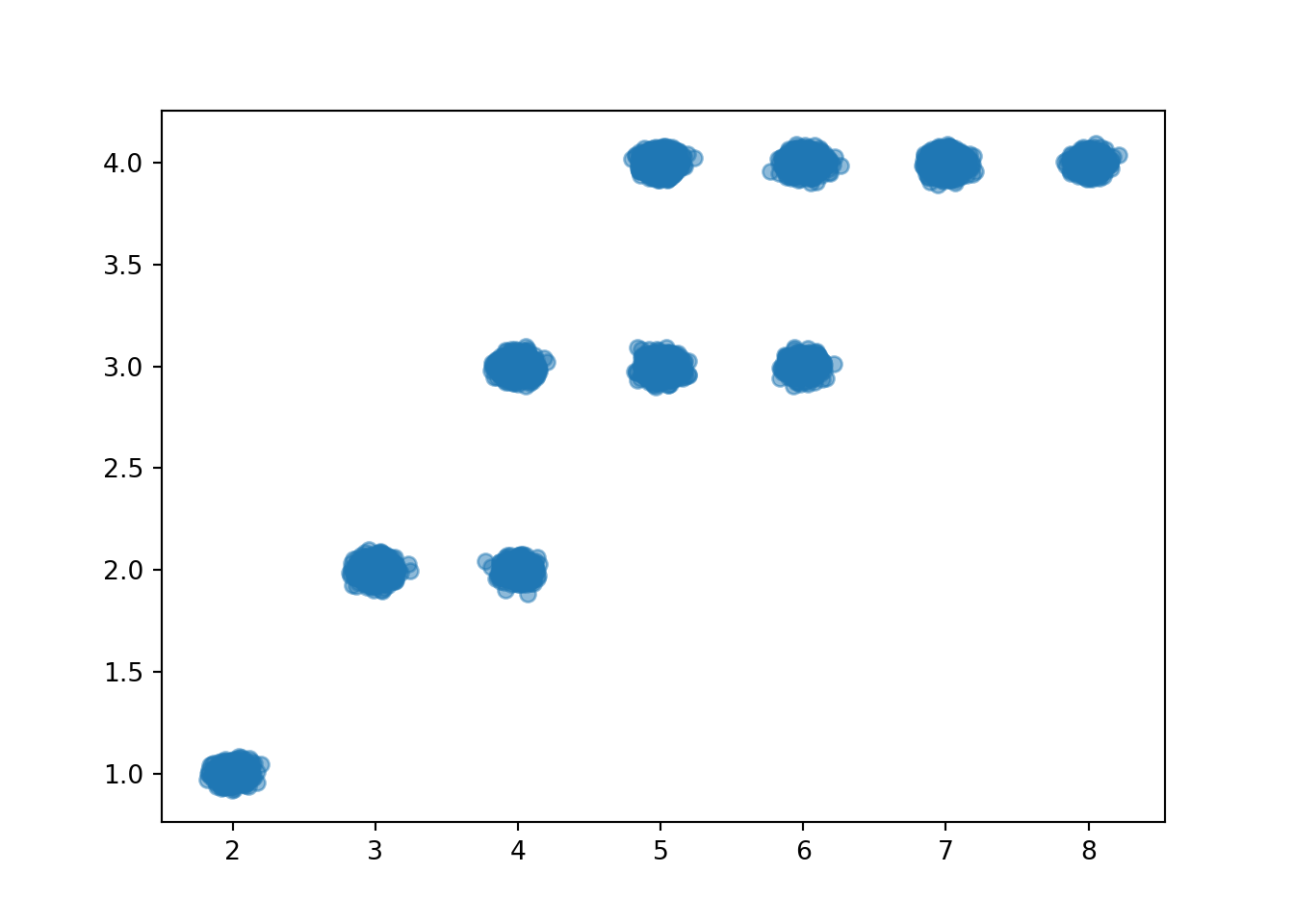

The tile plot provides a better summary. Notice how the colors represent the relative frequencies in the previous table.

x_and_y.plot('tile')

Finally, we find the simulated relative frequency of the event \(\{X <6, Y \ge 2\}\).

x_and_y.count(is_x_lt_6_and_y_ge_2) / x_and_y.count()

## 0.5632

Example 2.31 Recall the meeting problem. Use simulation to approximate the probability that Regina and Cady arrive with 15 minutes of each other for each of the three models in Section 2.5.3.

1. Uniform model
2. Normal model
3. Bivariate Normal model

Solution. to Example 2.31.

Show/hide solution

There are a few ways to code this, but it is easiest to define the waiting time variable \(W\) and find simulated relative frequencies of the event \(\{W<15\}\).

First the Uniform model.

P = Uniform(0, 60) ** 2
R, Y = RV(P)

W = abs(R - Y)

w = W.sim(10000)

w.count_lt(15) / w.count()

## 0.4349

Next the Normal model.

P = Normal(30, 10) ** 2
R, Y = RV(P)

W = abs(R - Y)

w = W.sim(10000)

w.count_lt(15) / w.count()

## 0.712

Finally the Bivariate Normal model.

P = BivariateNormal(mean1 = 30, sd1 = 10, mean2 = 30, sd2 = 10, corr = 0.7)
R, Y = RV(P)

W = abs(R - Y)

w = W.sim(10000)

w.count_lt(15) / w.count()

## 0.9488

We see that changing the assumptions changes the probability.

We’ll cover summarizing simulations of continuous random variables in much more detail later.

2.6.2 Approximating probabilities: Simulation margin of error

The probability of an event can be approximated by simulating the random phenomenon a large number of times and computing the relative frequency of the event. After enough repetitions we expect the simulated relative frequency to be close to the true probability, but there probably won’t be an exact match. Therefore, in addition to reporting the approximate probability, we should also provide a margin of error which indicates how close we think our simulated relative frequency is to the true probability.

Section 1.2.1 introduced the relative frequency interpretation in the context of flipping a fair coin. After many flips of a fair coin, we expect the proportion of flips resulting in H to be close to 0.5. But how many flips is enough? And how “close” to 0.5? We’ll investigate these questions now.

Consider Figure 2.18 below. Each dot represents a set of 10,000 fair coin flips. There are 100 dots displayed, representing 100 different sets of 10,000 coin flips each. For each set of flips, the proportion of the 10,000 flips which landed on head is recorded. For example, if in one set 4973 out of 10,000 flips landed on heads, the proportion of heads is 0.4973. The plot displays 100 such proportions; similar values have been “binned” together for plotting. We see that 98 of these 100 proportions are between 0.49 and 0.51, represented by the blue dots. So if “between 0.49 and 0.51” is considered “close to 0.5”, then yes, in 10000 coin flips we would expect⁵⁶ the proportion of heads to be close to 0.5.

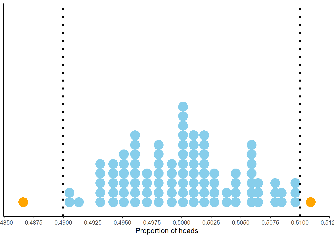
Figure 2.18: Proportion of flips which are heads in 100 sets of 10,000 fair coin flips. Each dot represents a set of 10,000 fair coin flips. In 98 of these 100 sets the proportion of heads is between 0.49 and 0.51 (the blue dots).

Our discussion of Figure 2.18 suggests that 0.01 might be an appropriate margin of error for a simulation based on 10,000 flips. Suppose we perform a simulation of 10000 flips with 4973 landing on heads. We could say “we estimate that the probability that a coin land on heads is equal to 0.4973”. But such a precise estimate would almost certainly be incorrect, due to natural variability in the simulation. In fact, only 0 sets⁵⁷ resulted in a proportion of heads exactly equal to the true probability of 0.5.

A better statement would be “we estimate that the probability that a coin land on heads is 0.4973 with a margin of error⁵⁸ of 0.01”. This means that we estimate that the true probability of heads is within 0.01 of 0.4973. In other words, we estimate that the true probability of heads is between 0.4873 and 0.5073, an interval whose endpoints are \(0.4973 \pm 0.01\). This interval estimate is “accurate” in the sense that the true probability of heads, 0.5, is between 0.4873 and 0.5073. By providing a margin of error, we have sacrificed a little precision — “equal to 0.4973” versus “within 0.01 of 0.4973” — to achieve greater accuracy.

Let’s explore this idea of “accuracy” further. Recall that Figure 2.18 displays the proportion of flips which landed on heads for 100 sets of 10000 flips each. Suppose that for each of these sets we form an interval estimate of the probability that the coin lands on heads by adding/subtracting 0.01 from the simulated proportion, as we did for \(0.4973 \pm 0.01\) in the previous paragraph. Figure 2.19 displays the results. Even though the proportion of heads was equal to 0.5 in only 0 sets, in 98 of these 100 sets (the blue dots/intervals) the corresponding interval contains 0.5, the true probability of heads. For almost all of the sets, the interval formed via “relative frequency \(\pm\) margin of error” provides an accurate estimate of the true probability. However, not all the intervals contain the true probability, which is why we often qualify that our margin of error is for “95% confidence” or “95% accuracy”. We will see more about “confidence” soon. In any case, the discussion so far, and the results in Figure 2.18 and Figure 2.19, suggest that 0.01 is a reasonable choice for margin of error when estimating the probability that a coin lands on heads based on 10000 flips.

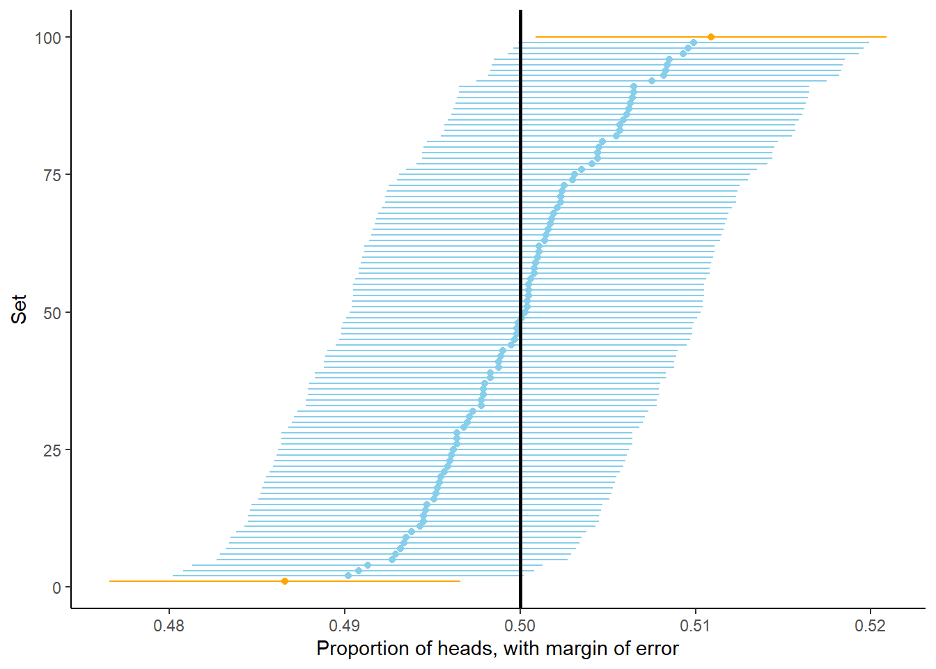
Figure 2.19: Interval estimates of the probability of heads based on 100 sets of 10,000 fair coin flips. Each dot represents the proportion of heads in a set of 10,000 fair coin flips. (The sets have been sorted based on their proportion of heads.) For each set an interval is obtained by adding/subtracting the margin of error of 0.01 from the proportion of heads. In 98 of these 100 sets (the blue dots/intervals) the corresponding interval contains the true probability of heads (0.5, represented by the vertical black line).

What if we want to be stricter about what qualifies as “close to 0.5”? That is, what if a margin of error of 0.01 isn’t good enough? You might suspect that with even more flips we would expect to observe heads on even closer to 50% of flips. Indeed, this is the case. Figure 2.20 displays the results of 100 sets of 1,000,000 fair coin flips. The pattern seems similar to Figure 2.18 but pay close attention to the horizontal axis which covers a much shorter range of values than in the previous figure. Now 95 of the 100 proportions are between 0.499 and 0.501. So in 1,000,000 flips we would expect⁵⁹ the proportion of heads to be between 0.499 and 0.501, pretty close to 0.5. This suggests that 0.001 might be an appropriate margin of error for a simulation based on 1,000,000 flips.

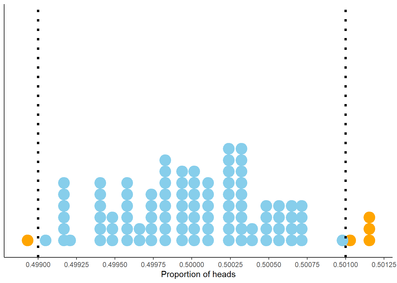
Figure 2.20: Proportion of flips which are heads in 100 sets of 1,000,000 fair coin flips. Each dot represents a set of 1,000,000 fair coin flips. In 95 of these 100 sets the proportion of heads is between 0.499 and 0.501 (the blue dots).

What about even more flips? In Figure 2.21 each dot represents a set of 100 million flips. The pattern seems similar to the previous figures, but again pay close attention the horizontal access which covers a smaller range of values. Now 93 of the 100 proportions are between 0.4999 and 0.5001. So in 100 million flips we would expect⁶⁰ the proportion of heads to be between 0.4999 and 0.5001, pretty close to 0.5. This suggests that 0.0001 might be an appropriate margin of error for a simulation based on 100,000,000 flips.

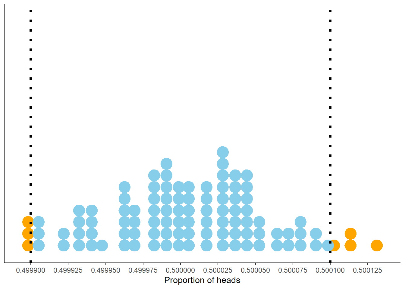
Figure 2.21: Proportion of flips which are heads in 100 sets of 100,000,000 fair coin flips. Each dot represents a set of 100,000,000 fair coin flips. In 93 of these 100 sets the proportion of heads is between 0.4999 and 0.5001 (the blue dots).

The previous figures illustrate that the more flips there are, the more likely it is that we observe a proportion of flips landing on heads close to 0.5. We also see that with more flips we can refine our definition of “close to 0.5”: increasing the number of flips by a factor of 100 (10,000 to 1,000,000 to 100,000,000) seems to give us an additional decimal place of precision (\(0.5\pm0.01\) to \(0.5\pm 0.001\) to \(0.5\pm 0.0001\).)

2.6.3 A closer look at margin of error

We will now carry out an analysis similar to the one above to investigate simulation margin of error and how it is influenced by the number of simulated values used to compute the relative frequency. Continuing the dice example, suppose we want to estimate \(p=\textrm{P}(X=6)\), the probability that the sum of two rolls of a fair four-sided equals six. Since there are 16 possible equally likely outcomes, 3 of which result in a sum of 3, the true probability is \(p=3/16=0.1875\).

We will perform a “meta-simulation”. The process is as follows

1. Simulate two rolls of a fair four-sided die. Compute the sum (\(X\)) and see if it is equal to 6.
2. Repeat step 1 to generate \(N\) simulated values of the sum (\(X\)). Compute the relative frequency of sixes: count the number of the \(N\) simulated values equal to 6 and divide by \(N\). Denote this relative frequency \(\hat{p}\) (read “p-hat”).
3. Repeat step 2 a large number of times, recording the relative frequency \(\hat{p}\) for each set of \(N\) values.

Be sure to distinguish between steps 2 and 3. A simulation will typically involve just steps 1 and 2, resulting in a single relative frequency based on \(N\) simulated values. Step 3 is the “meta” step; we see how this relative frequency varies from simulation to simulation to help us in determing an appropriate margin of error. The important quantity in this analysis is \(N\), the number of independently simulated values used to compute the relative frequency in a single simulation. We wish to see how \(N\) impacts margin of error. The number of simulations in step 3 just needs to be “large” enough to provide a clear picture of how the relative frequency varies from simulation to simulation. The more the relative frequency varies from simulation to simulation, the larger the margin of error needs to be.

We can combine steps 1 and 2 of the meta-simulation to put it in the framework of the simulations from earlier in this chapter. Namely, we can code the meta-simulation as a single simulation in which

• A sample space outcome represents \(N\) values of the sum of two fair-four sided dice
• The main random variable of interest is the proportion of the \(N\) values which are equal to 6.

Let’s first consider \(N=100\). The following Symbulate code defines the probability space corresponding to 100 values of the sum of two-fair four sided dice. Notice the use of apply which functions much in the same way⁶¹ as RV.

N = 100
P = BoxModel([1, 2, 3, 4], size = 2).apply(sum) ** N
P.sim(5)

Index	Result
0	(5, 6, 5, 3, 5, ..., 3)
1	(5, 4, 2, 6, 5, ..., 8)
2	(6, 5, 6, 5, 6, ..., 6)
3	(6, 4, 4, 5, 6, ..., 7)
4	(6, 5, 4, 6, 7, ..., 5)

In the code above

• BoxModel([1, 2, 3, 4], size = 2) simulates two rolls of a fair four-sided die
• .apply(sum) computes the sum of the two rolls
• ** N repeats the process n times to generate a set of N independent values, each value representing the sum of two rolls of a fair four-sided die
• P.sim(5) simulates 5 sets, each set consisting of N sums

Now we define the random variable which takes as an input a set of \(N\) sums and returns the proportion of the \(N\) sums which are equal to six.

phat = RV(P, count_eq(6)) / N
phat.sim(5)

Index	Result
0	0.17
1	0.18
2	0.23
3	0.2
4	0.19

In the code above

• phat is an RV defined on the probability space P. Recall that an outcome of P is a set of N sums (and each sum is the sum of two rolls of a fair four-sided die).
• The function that defines the RV is count.eq(6), which counts the number of values in the set that are equal to 6. We then⁶² divide by N, the total number of values in the set, to get the relative frequency. (Remember that a transformation of a random variable is also a random variable.)
• phat.sim(5) generates 5 simulated values of the relative frequency phat. Each simulated value of phat is the relative frequency of sixes in N sums of two rolls of a fair four-sided die.

Now we simulate and summarize a large number of values of phat. We’ll simulate 100 values for illustration (as we did in Figures 2.18, 2.20, and 2.21). Be sure not to confuse 100 with N. Remember, the important quantity is N, the number of simulated values used in computing each relative frequency.

plt.figure()
phat.sim(100).plot(type = "impulse", normalize = False)
plt.ylabel('Number of simulations');
plt.show()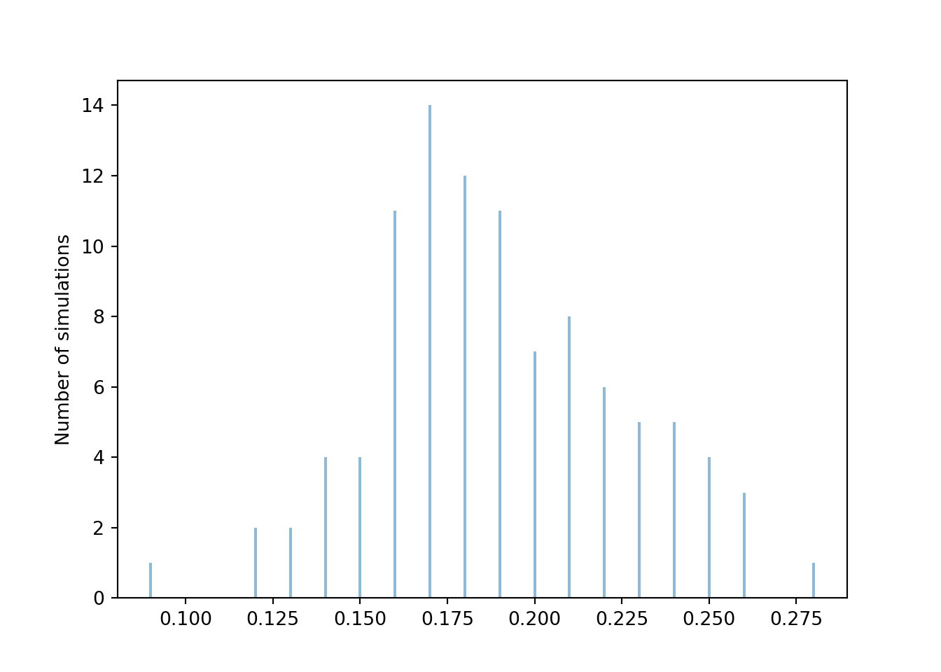

We see that the 100 relative frequencies are roughly centered around the true probability 0.1875, but there is variability in the relative frequencies from simulation to simulation. From the range of values, we see that most relative frequencies are within about 0.08 or so from the true probability 0.1875. So a value around 0.08 seems like a reasonable value of the margin of error, but the actual value depends on what we mean by “most”. We can get a clearer picture if we run more simulations. The following plot displays the results of 10000 simulations, each resulting in a value of \(\hat{p}\). Remember that each relative frequency is based on \(N=100\) sums of two rolls.

plt.figure()
phats = phat.sim(10000)
phats.plot(type = "impulse", normalize = False)
plt.ylabel('Number of simulations');
plt.show()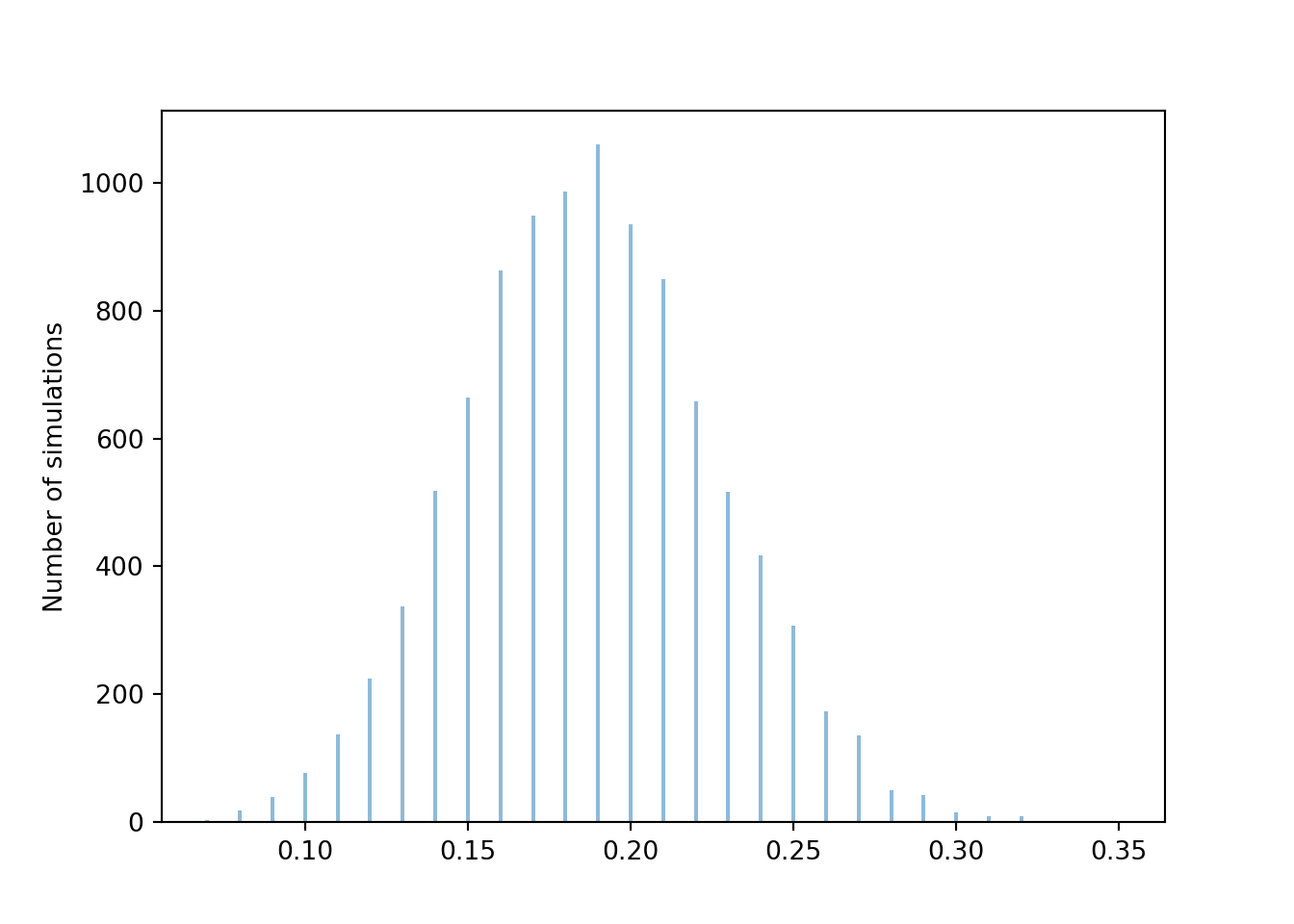

Let’s see how many of these 10000 simulated proportions are within 0.08 of the true probability 0.1875.

1 - (phats.count_lt(0.1875 - 0.08) + phats.count_gt(0.1875 + 0.08)) / 10000

## 0.9593

In roughly 95% or so of simulations, the simulated relative frequency was within 0.08 of the true probability. So 0.08 seems like a reasonable margin of error for “95% confidence” or “95% accuracy”. However, a margin of error of 0.08 yields pretty imprecise estimates, ranging from about 0.10 to 0.27. Can we keep the degree of accuracy at 95% but get a smaller margin of error, and hence a more precise estimate? Yes, if we increase the number of repetitions used to compute the relative frequency.

Now we repeat the analysis, but with \(N=10000\). In this case, each relative frequency is computed based on 10000 independent values, each value representing a sum of two rolls of a fair four-sided die. As before we start with 100 simulated relative frequencies.

N = 10000
P = BoxModel([1, 2, 3, 4], size = 2).apply(sum) ** N
phat = RV(P, count_eq(6)) / N

phats = phat.sim(100)
phats.plot(type = "impulse", normalize = False)
plt.ylabel('Number of simulations');
plt.show()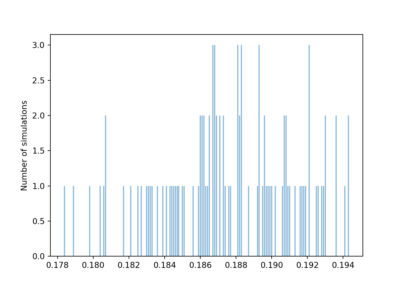

Again we see that the 100 relative frequencies are roughly centered around the true probability 0.1875, but there is less variability in the relative frequencies from simulation to simulation for \(N=10000\) than for \(N=100\). Pay close attention to the horizontal axis. From the range of values, we see that most relative frequencies are now within about 0.008 of the true probability 0.1875.

1 - (phats.count_lt(0.1875 - 0.008) + phats.count_gt(0.1875 + 0.008)) / 100

## 0.98

As with \(N=100\), running more than 100 simulations would give a clearer picture of how much the relative frequency based on \(N=10000\) simulated values varies from simulation to simulation. But even with just 100 simulations, we see that a margin of error of about 0.008 is required for roughly 95% accuracy when \(N=10000\), as opposed to 0.08 when \(N=100\). As we observed in the coin flipping example earlier in this section, it appears that increasing \(N\) by a factor of 100 yields an extra decimal place of precision. That is, increasing \(N\) by a factor of 100 decreases the margin of error by a factor of \(\sqrt{100}\). In general, the margin of error is inversely related to \(\sqrt{N}\).

Table 2.20: Comparison of margins of error for 95% confidence for the meta-simulations in this section.

Probability that	True value	95% m.o.e. (N = 100)	95% m.o.e. (N = 10000)	95% m.o.e. (N = 1000000)
A fair coin flip lands H	0.5000	0.1000	0.0100	1e-03
Two rolls of a fair four-sided die sum to 6	0.1875	0.0781	0.0078	8e-04

The two examples in this section illustrate that the margin of error also depends somewhat on the true probability. The margin of error required for 95% accuracy is larger when the true probability is 0.5 than when it is 0.1875. It can be shown that when estimating a probability \(p\) with a relative frequency based on \(N\) simulated repetitions, the margin of error required for 95% confidence⁶³ is \[ 2\frac{\sqrt{p(1-p)}}{\sqrt{N}} \] For a given \(N\), the above quantity is maximized when \(p\) is 0.5. Since \(p\) is usually unknown — the reason for performing the simulation is to approximate it — we plug in 0.5 for a somewhat conservative margin of error of \(1/\sqrt{N}\).

For a fixed \(N\), there is a tradeoff between accuracy and precision. The factor 2 in the margin of error formula above corresponds to 95% accuracy. Greater accuracy would require a larger factor, and a larger margin of error, resulting in a wider — that is, less precise — interval. For example, 99% confidence requires a factor of roughly 2.6 instead of 2, resulting in an interval that is roughly 30 percent wider. The confidence level does matter, but the primary influencer of margin of error is \(N\), the number of repetitions on which the relative frequency is based. Regardless of confidence level, the margin of error is on the order of magnitude of \(1/\sqrt{N}\).

In summary, the margin of error when approximating a probability based on a simulated relative frequency is roughly on the order \(1/\sqrt{N}\), where \(N\) is the number of independently simulated values used to calculate the relative frequency. Warning: alternative methods are necessary when the actual probability being estimated is very close to 0 or to 1.

A probability is a theoretical long run relative frequency. A probability can be approximated by a relative frequency from a large number of simulated repetitions, but there is some simulation margin of error. Likewise, the average value of \(X\) after a large number of simulated repetitions is only an approximation to the theoretical long run average value of \(X\). The margin of error is also on the order of \(1/\sqrt{N}\) where \(N\) is the number of simulated values used to compute the average. We will explore margins of error for long run averages in more detail later.

Pay attention to the wording: \(N\) is the number of independently⁶⁴ simulated values used to calculate the relative frequency. This is not necessarily the number of simulated values. For example, suppose we use simulation to approximate the probability that the larger of two rolls of a fair four-sided die is 4 when the sum is equal to 6. We might start by simulating 10000 pairs of rolls. But the sum would be equal to 6 in only about 1875 pairs, and it is only these pairs that would be used to compute the relative frequency that the larger roll is 4 to approximate the probability of interest. The appropriate margin of error is roughly \(1/\sqrt{1875} \approx 0.023\). Compared to 0.01 (based on the original 10000 repetitions) the margin of error of 0.023 results in intervals that are 130 percent wider. Carefully identifying the number of values used to calculate the relative frequency is especially important when determining appropriate simulation margins of error for approximating conditional probabilities, which we’ll discuss in more detail later.

2.6.4 Approximating multiple probabilities

When using simulation to estimate a single probability, the primary influencer of margin of error is \(N\), the number of repetitions on which the relative frequency is based. It doesn’t matter as much whether we use, say, 95% versus 99% confidence. That is, it doesn’t matter too much whether we compute our margin of error using \[ 2\frac{\sqrt{p(1-p)}}{\sqrt{N}}, \] with a multiple of 2 for 95% confidence, or if we replace 2 by 2.6 for 99% confidence. (Remember, we can plug in 0.5 for the unknown \(p\) for a conservative margin of error.) A margin of error based on 95% or 99% (or another confidence level in the neighborhood) provides a reasonably accurate estimate of the probability. However, using simulation to approximate multiple probabilities simultaneously requires a little more care with the confidence level.

In the previous section we used simulation to estimate \(\textrm{P}(X=6)\). Now suppose we want to approximate \(\textrm{P}(X = x)\) for each value of \(x = 2,3,4,5,6,7,8\). We could run a simulation like the one in Section ?? to obtain results like those in Figure 2.16 and the table before it. Each of the relative frequencies in the table is an approximation of the true probability, and so each of the relative frequencies should have a margin of error, say 0.01 for a simulation based on 10000 repetitions. Thus, the simulation results yield a collection of seven interval estimates, an interval estimate of \(\textrm{P}(X = x)\) for each value of \(x = 2,3,4,5,6,7,8\). Each interval in the collection either contains the respective true probability or not. The question is then: In what percent of simulations will every interval in the collection contain the respective true probability?

Figure 2.22 summarizes the results of 100 simulations. Each simulation consists of 10000 repetitions, with results similar to those in Figure 2.16 and the table before it. Each simulation is represented by a row in Figure 2.22, consisting of seven 95% interval estimates, one for each value of \(x\). Each panel represents a different value of \(x\); for each value of \(x\), around 95 out of the 100 simulations yield estimates that contain the true probability \(\textrm{P}(X=x)\), represented by the vertical line.

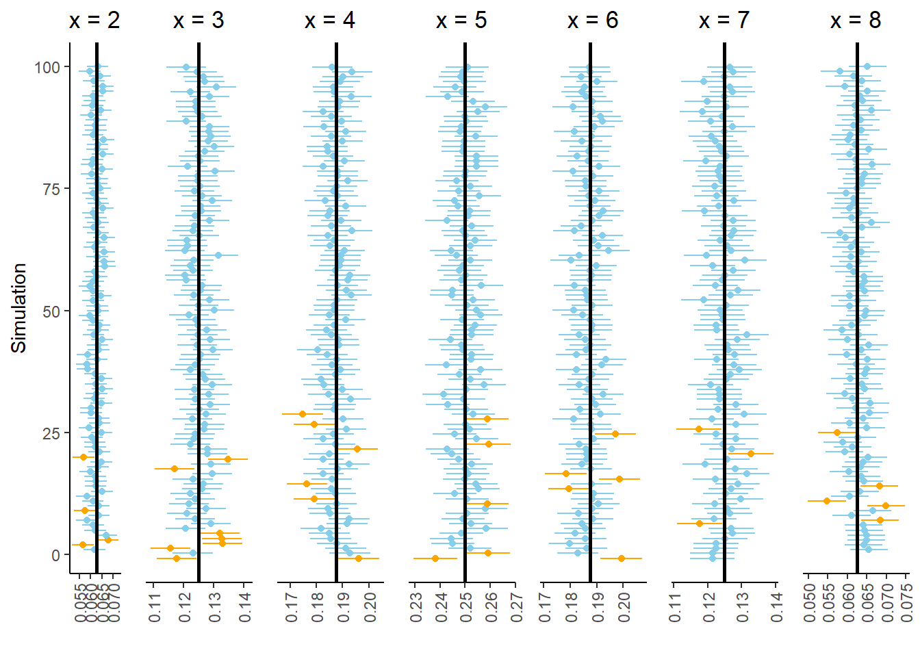
Figure 2.22: Results of 100 simulations. Each simulation yields a collection of seven 95% confidence intervals.

However, let’s zoom in on the bottom of Figure 2.22. Figure 2.23 displays the results of the 30 simulations at the bottom of Figure 2.22. Look carefully row by row in Figure 2.23; in each of these simulations at least one of the seven intervals in the collection does not contain the true probability. In other words, every interval in the collection contains the respective true probability in only 70 of the 100 simulations (the other simulations in Figure 2.22.) While we have 95 percent confidence in our interval estimate of \(\textrm{P}(X = x)\) for any single \(x\), we only have around 70 percent confidence in our approximate distribution of \(X\). Our confidence “grade” has gone from A range (95 percent) to C range (70 percent).

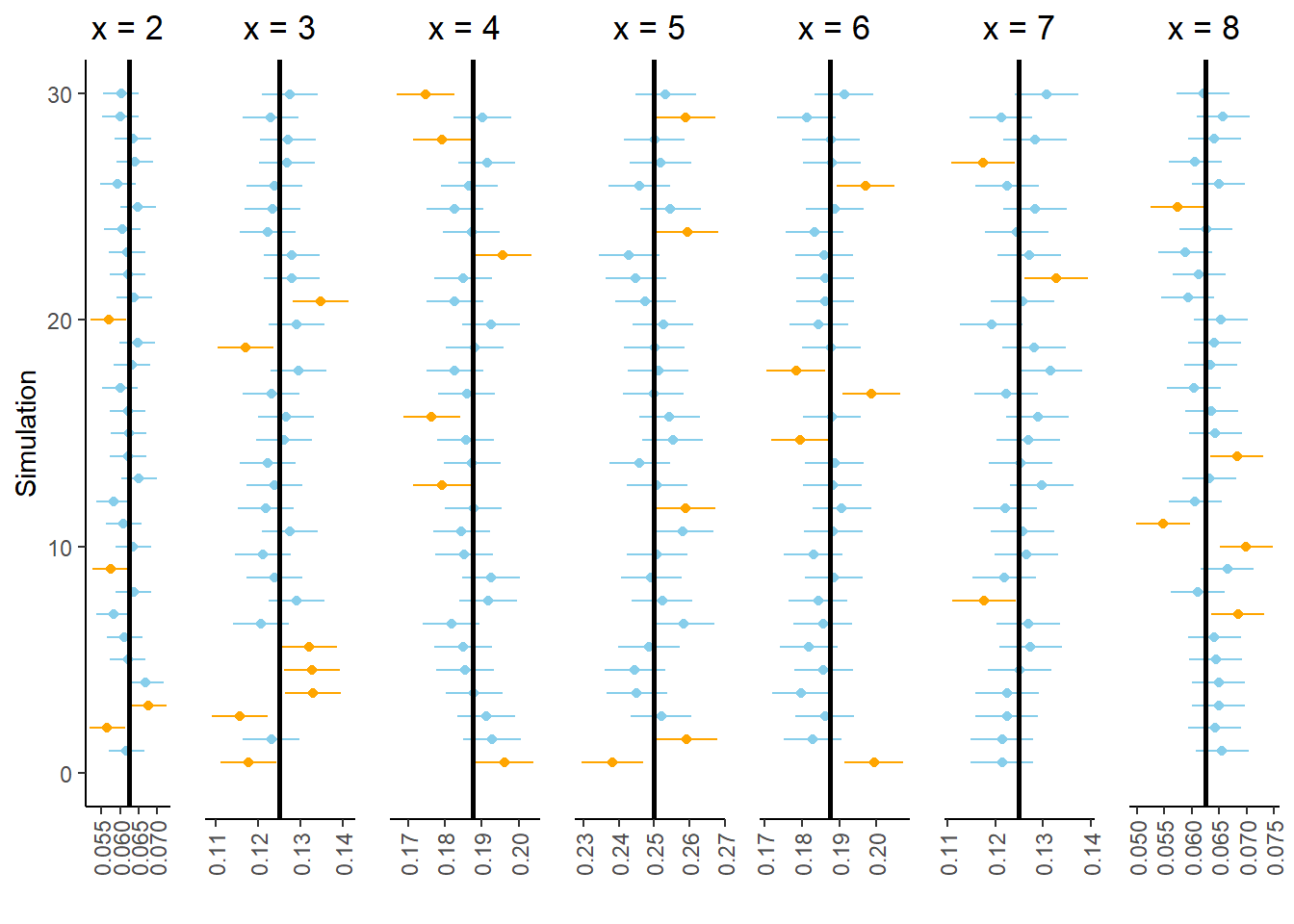
Figure 2.23: Subset of 30 simulations from Figure 2.22. In each of these simulations, at least one 95% confidence interval does not contain the respective true probability.

When approximating multiple probabilities based on a single simulation, such as when approximating a distribution, margins of error and interval estimates need to be adjusted to obtain simultaneous 95% confidence. The easiest way to do this is to make all of the intervals in the collection wider.

There are many procedures for adjusting a collection of interval estimates to achieve simultaneous confidence; we won’t get into any technical details. As a very rough, but simple and typically conservative rule, when approximating many probabilities based on a single simulation, we recommend making the margin of error twice as large as when approximating a single probability. That is, use a margin of error of \(2/\sqrt{N}\) (rather than \(1/\sqrt{N}\)) to achieve simultaneous 95% confidence when approximating many probabilities based on a single simulation.

2.6.5 Beware a false sense of precision

Why don’t we always run something like one trillion repetitions so that our margin of error is tiny? There is a cost to simulating and storing more repetitions in terms of computational time and memory. Also, remember that simulating one trillion repetitions doesn’t guarantee that the margin of error is actually based on anywhere close to one trillion repetitions, especially when conditioning on a low probability event.

Most importantly, keep in mind that any probability model is based on a series of assumptions and these assumptions are not satisfied exactly by the random phenomenon. A precise estimate of a probability under the assumptions of the model is not necessarily a comparably precise estimate of the true probability. Reporting probability estimates out to many decimal places conveys a false sense of precision and should typically be avoided.

For example, the probability that any particular coin lands on heads is probably not 0.5 exactly. But any difference between the true probability of the coin landing on heads and 0.5 is likely not large enough to be practically meaningful⁶⁵. That is, assuming the coin is fair is a reasonable model.

Suppose we assume that the probability that a coin lands on heads is exactly 0.5 and that the results of different flips are independent. If we flip the coin 1000 times the probability that it lands on heads at most 490 times is 0.2739864. (We will see a formula for computing this value later.) If we were to simulate one trillion repetitions (each consisting of 1000 flips) to estimate this probability then our margin of error would be 0.000001; we could expect accuracy out to the sixth decimal place. However, reporting the probability with so many decimal places is somewhat disingenuous. If the probability that the coin lands on heads were 0.50001, then the probability of at most 490 heads in 1000 flips would be 0.2737757. If the probability that the coin lands on heads were 0.5001, then the probability of at most 490 heads in 1000 flips would be 0.2718834. Reporting our approximate probability as something like 0.2739864 \(\pm\) 0.000001 says more about the precision in our assumption that the coin is fair than it does about the true probability that the coin lands on heads at most 490 times in 1000 flips. A more honest conclusion would result from running 10000 repetitions and reporting our approximate probability as something like 0.27 \(\pm\) 0.01. Such a conclusion reflects more genuinely that there’s some “wiggle room” in our assumptions, and that any probability computed according to our model is at best a reasonable approximation of the “true” probability.

For most of the situations we’ll encounter in this book, estimating a probability to within 0.01 of its true value will be sufficient for practical purposes, and so basing approximations on 10000 simulated values will be appropriate. Of course, there are real situations where probabilities need to be estimated much more precisely, e.g., the probability that a bridge will collapse. Such situations require more intensive methods.

---

52. Do we perform “a simulation”, or “many simulations”? Throughout, “a simulation” refers to the collection of results corresponding to repeatedly artificially recreating the random process. “A repetition” refers to a single artificial recreation resulting in a single simulated outcome. We perform a simulation which consists of many repetitions.↩︎

53. We would typically only include the values observed in the simulation in the summary. However, we include 4 and 8 here because if we had performed more repetitions we would have observed these values.↩︎

54. “Normalize” is used in the sense of Section 1.3 and refers to rescaling the values so that they add up to 1 but the ratios are preserved.↩︎

55. For discrete random variables 'impulse' is the default plot type. Like .tabulate(), the .plot() method also has a normalize argument; the default is normalize=True.↩︎

56. In 10000 flips, the probability of heads on between 49% and 51% of flips is 0.956, so 98 out of 100 provides a rough estimate of this probability. We will see how to compute such a probability later.↩︎

57. This is difficult to see in Figure 2.18 due to the binning. But we can at least tell from Figure 2.18 that at most a handful of the 100 sets resulted in a proportion of heads exactly equal to 0.5.↩︎

58. Technically, we should say “a margin of error for 95% confidence of 0.01”. We’ll discuss “confidence” in a little more detail soon.↩︎

59. In 1,000,000 flips, the probability of heads on between 49.9% and 50.1% of flips is 0.955, and 95 out of 100 sets provides a rough estimate of this probability.↩︎

60. In 100 million flips, the probability of heads on between 49.99% and 50.01% of flips is 0.977, and 93 out of 100 sets provides a rough estimate of this probability.↩︎

61. One difference between RV and apply: apply preserves the type of the input object. That is, if apply is applied to a ProbabilitySpace then the output will be a ProbabilitySpace; if apply is applied to an RV then the output will be an RV. In contrast, RV always creates an RV.↩︎

62. Unfortunately, for techincal reasons, RV(P, count_eq(6) / N) will not work. It is possible to divide by N within RV if we define a custom function def rel_freq_six(x): return x.count_eq(6) / N and then define RV(P, rel_freq_six).↩︎

63. We will see the rationale behind this formula later. The factor 2 comes from the fact that for a Normal distribution, about 95% of values are within 2 standard deviations of the mean. Technically, the factor 2 corresponds to 95% confidence only when a single probability is estimated. If multiple probabilities are estimated simultaneously, then alternative methods should be used, e.g., increasing the factor 2 using a Bonferroni correction. For example, a multiple of 4 rather than 2 produces very conservative error bounds for 95% confidence even when many probabilities are being estimated.↩︎

64. In all the situations in this book the values will be simulated independently. However, there are many simulation methods where this is not true, most notably MCMC (Markov Chain Monte Carlo) methods. The margin of error needs to be adjusted to reflect any dependence between simulated values.↩︎

65. There is actually some evidence that a coin flip is slightly more likely to land the same way it started; e.g, a coin that starts H up is more likely to land H up. But the tendency is small.↩︎