6.2 Binomial distributions

We introduced Binomial distributions in Section 4.2.3. Now we’ll study Binomial distributions in more detail. Our first example is just to remind us of situations where Binomial distributions arise.

Example 6.2 Consider an extremely simplified model for the daily closing price of a certain stock. Every day the price either goes up or goes down, and the movements are independent from day-to-day. Assume that the probability that the stock price goes up on any single day is 0.25. Let $X$ be the number of days in which the price goes up in the next 5 days.

Compute and interpret $\textrm{P}(X=5)$.
Compute the probability that the price goes up on the next three days and then down on the following two days.
Compute and interpret $\textrm{P}(X=3)$. Why is $\textrm{P}(X=3)$ different from the probability in the previous part?
Suggest a general formula for the probability mass function of $X$.
Use the pmf of $X$ to construct a table, plot, and spinner of the distribution of $X$.
Suggest a “shortcut” formula for $\textrm{E}(X)$. Then use the table from the previous part to compute $\textrm{E}(X)$. Did the shortcut formula work? Interpret $\textrm{E}(X)$.
Is the random variable $X$ in this problem the same random variable as the random variable $X$ in 4.8?
Does the random variable $X$ in this problem have the same distribution the random variable $X$ in 4.8?

Solution. to Example 6.2

Show/hide solution

Days are independent so we can multiply probabilities \[ \textrm{P}(X = 5) = (0.25)(0.25)(0.25)(0.25)(0.25) = (0.25)^5 = \binom{5}{5}(0.25)^5(1-0.25)^{5 -5} = 0.00098 \] In about 0.098% of 5-day periods the price goes up all 5 days.
Days are independent so we can multiply probabilities \[ (0.25)(0.25)(0.25)(1-0.25)(1-0.25) = (0.25)^3(1-0.25)^{5-3} = 0.0088 \]
SSSFF is only one outcome with $X=3$. There are $\binom{5}{3}=10$ total outcomes for which $X = 3$, each with probability $(0.25)^3(1-0.25)^2$, so \[ \textrm{P}(X = 3) = 10(0.25)^3(1-0.25)^2 = \binom{5}{3}(0.25)^3(1-0.25)^{5-3} = 0.088 \] In about 8.8% of 5-day periods the price goes up on exactly 3 of the 5 days.
The pmf is \[ p(x) = \begin{cases} \binom{5}{x} 0.25^x (1-0.25)^{5-x}, & x=0, 1, 2, 3, 4, 5\\ 0, & \text{otherwise} \end{cases} \]
See Example 4.8 and the discussion following it.
If price goes up on 25% of days we would expect $5(0.25) = 1.25$ up movements in 5 days, on average in the long run. This is what we get if we compute the expected value the “long way” based on the distribution table.
These are different random variables. The number of tagged butterflies is different than the number of up price movements.
Yes, they have the same distribution. While the contexts are different and the variables are measuring different things, probabilistically the situations are equivalent. In each situation:
- There are S/F trials (tagged/not, up/not)
- Trials are independent (sampling with replacement, by assumption)
- Probability of success of 0.25 on each trial (13/52, assumed 0.25)
- 5 trials (5 butterflies, 5 days)
- $X$ counts the number of successes (number of tagged butterflies, number of up movements) Therefore, in each problem the random variable $X$ has a Binomial(5, 0.25) distribution.

Definition 6.2 A discrete random variable $X$ has a Binomial distribution with parameters $n$, a nonnegative integer, and $p\in[0, 1]$ if its probability mass function is \[\begin{align*} p_{X}(x) & = \binom{n}{x} p^x (1-p)^{n-x}, & x=0, 1, 2, \ldots, n \end{align*}\] If $X$ has a Binomial($n$, $p$) distribution \[\begin{align*} \textrm{E}(X) & = np\\ \textrm{Var}(X) & = np(1-p) \end{align*}\]

Imagine a box containing tickets with $p$ representing the proportion of tickets in the box labeled 1 (“success”); the rest are labeled 0 (“failure”). Randomly select $n$ tickets from the box with replacement and let $X$ be the number of tickets in the sample that are labeled 1. Then $X$ has a Binomial($n$, $p$) distribution. Since the tickets are labeled 1 and 0, the random variable $X$ which counts the number of successes is equal to the sum of the 1/0 values on the tickets. If the selections are made with replacement, the draws are independent, so it is enough to just specify the population proportion $p$ without knowing the population size $N$.

The situation in the previous paragraph and example involves a sequence of Bernoulli trials.

There are only two possible outcomes, “success” (1) and “failure” (0), on each trial.
The unconditional/marginal probability of success is the same on every trial, and equal to $p$
The trials are independent.

If $X$ counts the number of successes in a fixed number, $n$, of Bernoulli($p$) trials then $X$ has a Binomial($n, p$) distribution.
Careful: Don’t confuse the number $p$, the probability of success on any single trial, with the probability mass function $p_X(\cdot)$ which takes as an input a number $x$ and returns as an output the probability of $x$ successes in $n$ Bernoulli($p$) trials, $p_X(x)=\textrm{P}(X=x)$.

Example 6.3 Continuing Example 6.3.

What does the random variable $5-X$ represent? What is its distribution?
Suppose that the price is currently $100 and each it either moves up $2 or down $2. Let $S$ be the stock price after 5 days. How does $S$ relate to $X$? Does $S$ have a Binomial distribution?
Recall that $X$ is the number of days on which the price goes up in the next five days. Suppose that $Y$ is the number of days on which the price goes up in the ten days after that (days 6-15). What is the distribution of $X+Y$? (Continue to assume independence between days, with probability 0.25 of an up movement on any day.)

Solution. to Example 6.3

Show/hide solution

Since on each day the price either moves up or down, if $X$ is the number of days the price moves up, then $5-X$ is the number of days the price moves down. $5-X$ counts down days, so just change the “success/failure” labels; now “success” is down, and the probability of down on any single day is 0.75. So the distribution of $5-X$ is Binomial(5, 0.75).
$S = 100 + 2X -2(5-X) = 4X + 90$. $S$ is a linear rescaling, so it doesn’t change the basic shape of the distribution. However, technically $S$ does not have a Binomial distribution, because the possible values of a variable with a Binomial distribution are always $0, 1, \ldots, n$. The distribution of $S$ is like a “rescaled” Binomial distribution.
$X+Y$ is the total number of up days in the 15 days. The Binomial situation is still satisfied, but now with $n=15$, so $X+Y$ has a Binomial(15, 0.25) distribution.

Example 6.4 In each of the following situations determine whether or not $X$ has a Binomial distribution. If so, specify $n$ and $p$. If not, explain why not.

Roll a die 20 times; $X$ is the number of times the die lands on an even number.
Roll a die 20 times; $X$ is the number of times the die lands on 6.
Roll a die until it lands on 6; $X$ is the total number of rolls.
Roll a die until it lands on 6 three times; $X$ is the total number of rolls.
Roll a die 20 times; $X$ is the sum of the numbers rolled.
Shuffle a standard deck of 52 cards (13 hearts, 39 other cards) and deal 5 without replacement; $X$ is the number of hearts dealt. (Hint: be careful about why.)
Roll a fair six-sided die 10 times and a fair four-sided die 10 times; $X$ is the number of 3s rolled (out of 20).

Solution. to Example 6.4

Show/hide solution

Yes, Binomial(20, 0.5). Success = even.
Yes, Binomial(20, 1/6). Success = 6. (The probability of success has to be the same on each trial. However, the probability of success does not have to be the same as the probability of failure.)
Not Binomial; not a fixed number of trials. These are Bernoulli trials, but the random variable is not counting the number of successes in a fixed number of trials.
Not Binomial; not a fixed number of trials. These are Bernoulli trials, but the random variable is not counting the number of successes in a fixed number of trials.
Not Binomial; each trial has more outcomes than just success or failure, and the random variable is summing the values rather than counting successes.
Not Binomial, because the trials are not independent. The conditional probability that the second card is a heart given that the first card is a heart is 12/51, which is not equal to the conditional probability that the second card is a heart given that the first card is not a heart, 13/51. The trials are not independent. However, the unconditional probability of success is the same on each trial, $p=13/52$. Recall Section 3.4.
Not Binomial. Here the trials are independent, but the probability of success is not the same on each trial; it’s 1/6 for the six-sided die trials but 1/4 for the four sided-die trials.

Do not confuse the following two distinct assumptions of Bernoulli trials.

The probability of success is the same on each trial — this concerns the unconditional/marginal probability of each individual trial.
- The probability of success will be the same on each trial regardless of whether the sampling is with or without replacement as long as all trials are sampled from the same population.
The trials are independent — this concerns joint or conditional probabilities for the collection of trials.
- The trials will technically only be independent if the sampling is with replacement.
- But when sampling without replacement, if the population size is much larger than the sample size then the trials will be nearly independent.

Example 6.5 Each of the plots below displays a Binomial distribution with $p=0.4$ (and different values of $n$). For a fixed value of $p$, how does the variance of a Binomial distribution relate to $n$? (Note: the plots are on the same scale, so some probabilities are 0.)


p = 0.4

ns = [5, 10, 15, 20]

for n in ns:
  Binomial(n, p).plot()

plt.legend(ns, title = "n")

plt.show()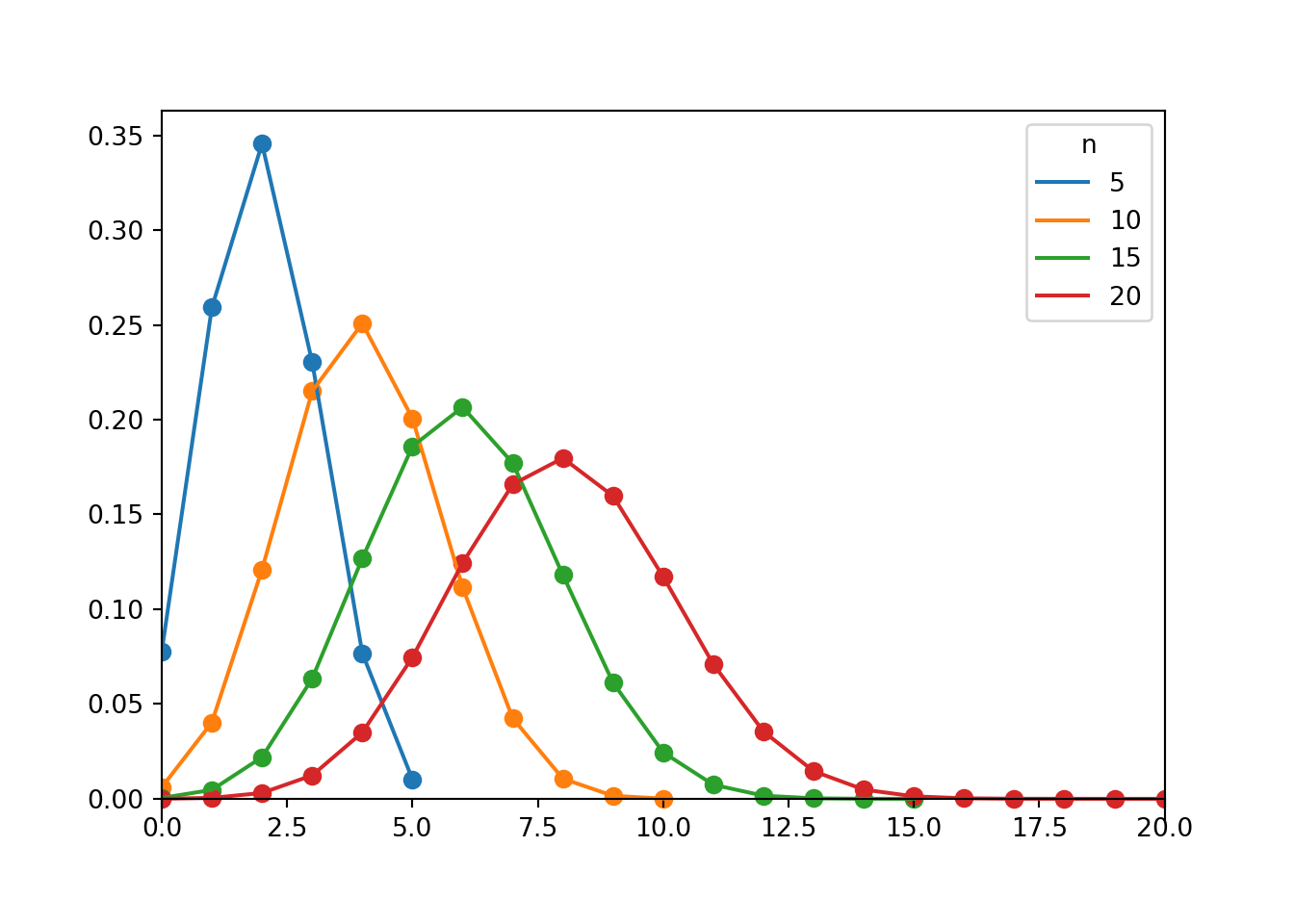

$Probability mass functions for Binomial($n$, 0.4) distributions for $n = 5, 10, 15, 20$.$

Figure 6.1: Probability mass functions for Binomial($n$, 0.4) distributions for $n = 5, 10, 15, 20$.

Solution. to Example 6.5

Show/hide solution

For a Binomial($n$, $p$) distribution, variance increases as $n$ increases. Since the possible values of a random variable with a Binomial distribution are $0, 1, \ldots, n$, as $n$ increases the range of possible values of the variable increases.

However, in some sense it is unfair to compare values from Binomial distributions with different values of $n$. Ten successes has a very different meaning if $n$ is 10 or 20 or 100. Rather than focusing on the absolute number of successes, in Binomial situations we are often concerned with the proportion of successes in the sample. We will see soon that as the sample size $n$ increases, the variance of the sample proportion decreases.

Example 6.6 Each of the plots below displays a Binomial distribution with $n=10$ (and different values of $p$). For a fixed value of $n$, how does the variability of a Binomial distribution relate to $p$? (Note the values which have essentially 0 probability.)


n = 10

ps = [0.1, 0.3, 0.5, 0.7, 0.9]

for p in ps:
  Binomial(n, p).plot()

plt.legend(ps, title = "p", loc = "upper center");
plt.xlim(-0.2, n + 0.2)

## (-0.2, 10.2)

plt.show()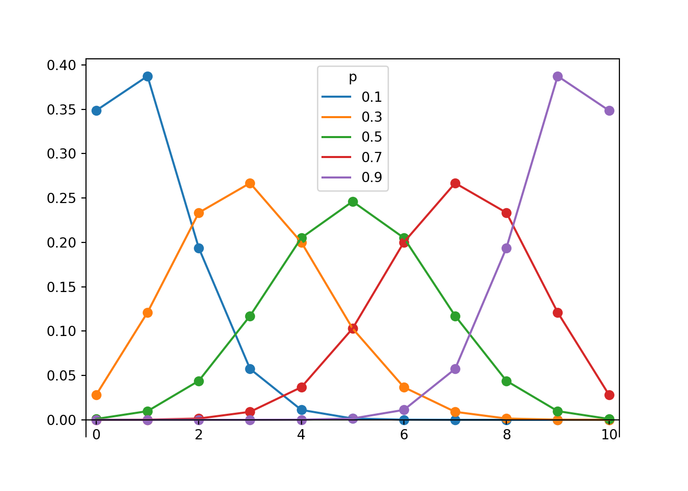

$Probability mass functions for Binomial(10, $p$) distributions for $p = 0.1, 0.3, 0.5, 0.7, 0.9$.$

Figure 6.2: Probability mass functions for Binomial(10, $p$) distributions for $p = 0.1, 0.3, 0.5, 0.7, 0.9$.

Solution. to Example 6.6

Show/hide solution

The distribution is most disperse, and the variance largest, when $p=0.5$. When $p=0.5$ we would expect the most “alterations” between success and failure in the individual trials.

Variance decreases as $p$ moves away from 0.5. That is, variance decreases as $p$ gets closer to 0 or 1. The variance when $p=0.3$ appears to be the same as when $p=0.7$, and similarly for $p=0.1$ and $p=0.9$. For the extreme case $p=0$, every trials results in failure so the number of successes is always 0 and the variance is 0. Likewise, when $p=1$ every trials results in success so the number of successes is always $n$, and the variance is 0.

The previous exercises provide an intuitive explanation of the formula for the variance of a Binomial distribution: $\textrm{Var}(X) = np(1-p)$. The formula can be derived using indicators and the fact that a sum of independent random variables is the sum of the variances.

Example 6.7 Suppose there are 21,812 students at Cal Poly, 18,388 of whom are CA residents. Select a random sample of 35 Cal Poly students, and let $X$ be the number of CA residents in the sample.

Identify the distribution of $X$, its variance, and $\textrm{P}(X\le 27)$ if the sampling is performed with replacement.
Identify the distribution of $X$, its variance, and $\textrm{P}(X\le 27)$ if the sampling is performed without replacement.

Solution. See the code and output below. The values are virtually identical regardless of whether the sampling is performed with or without replacement.


RV(Binomial(35, 18388 / 21812)).sim(100000).plot()
Hypergeometric(n = 35, N1 = 18388, N0 = 21812 - 18388).plot()
plt.xlim(20, 36);
plt.show()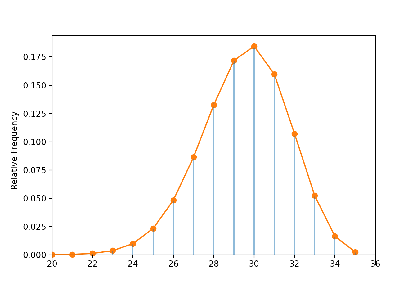


Binomial(35, 18388 / 21812).cdf(27), Hypergeometric(n = 35, N1 = 18388, N0 = 21812 - 18388).cdf(27)

## (0.1731226433484683, 0.1729547901612607)


Binomial(35, 18388 / 21812).var(), Hypergeometric(n = 35, N1 = 18388, N0 = 21812 - 18388).var()

## (4.631752209981104, 4.624532019474508)

Consider a finite “success/failure” population of size $N$ in which the population proportion of success is $p$. Suppose a random sample of size $n$ is selected without replacement and $X$ is the number of successes in the sample. If the population size $N$ is much larger than the sample size $n$, then

the selections are “nearly” independent
$p_X(x)\approx \binom{n}{x}p^x(1-p)^{n-x}$
$\textrm{Var}(X)\approx np(1-p)$

That is, if the population size $N$ is much larger than the sample size $n$, a Hypergeometric distribution is closely approximated by a corresponding Binomial distribution. (We will see soon that a Binomial distribution is often closely approximated by either a Poisson distribution or a Normal distribution).

Example 6.8 Let $X_1$ and $X_2$ be independent random variables and suppose that $X_1$ has a Binomial($n_1$, $p$) distribution and $X_2$ has a Binomial($n_2$, $p$) (Note that $p$ is the same.) Use a “story proof” to find the distribution of $X_1+X_2$ without any calculations

Solution. to Example 6.8

Show/hide solution

Suppose $X_1$ counts the number of successes in $n_1$ Bernoulli($p$) trials, and $X_2$ counts the number of successes in $n_2$ Bernoulli($p$) trials. The two sets of trials are independent since $X_1$ and $X_2$ are. Then $X_1+X_2$ counts the total number of successes in $n_1+n_2$ Bernoulli($p$) trials. Therefore $X_1+X_2$ has a Binomial($n_1+n_2$, $p$) distribution.

A Binomial(1, $p$) distribution is also known as a Bernoulli($p$) distribution, taking a value of 1 with probability $p$ and 0 with probability $1-p$. Any indicator random variable has a Bernoulli distribution.

If $X_1, X_2, \ldots, X_n$ are independent each with a Bernoulli($p$) distribution, then $X_1+\cdots+X_n$ has a Binomial($n, p$) distribution. So any random variable with a Binomial($n$, $p$) distribution has the same distributional properties as $X_1+ X_2+ \cdots+ X_n$, where $X_1, \ldots, X_n$ are independent each with a Bernoulli($p$) distribution. This provides a very convenient representation in many problems.

Example 6.9 Continuing Example 4.8. Define the random variable $\hat{p} = X/5$.

What does $\hat{p}$ represent in this context. What are its possible values?
Does $\hat{p}$ have a Binomial distribution? Does the distribution of $\hat{p}$ have the same basic shape of a Binomial distribution?
Compute $\textrm{P}(\hat{p} = 0.2)$.
Compute $\textrm{E}(\hat{p})$. Why does this make sense?
Compute $\textrm{SD}(\hat{p})$.
Suppose that 20 butterflies were selected for the second sample at random, with replacement. Compute $\textrm{SD}(\hat{p})$; how does the value compare to the previous part?

Solution. to Example 6.9

Show/hide solution

$\hat{p}$ is the proportion of butterflies in the second sample that are tagged. Possible values are 0, 1/5, 2/5, 3/5, 4/5, 1.
Technically $\hat{p}$ does not have a Binomial distribution, since a Binomial distribution always corresponds to possible values 0, 1, 2, $\ldots, n$. But the distribution of $\hat{p}$ does follow the same shape as the Binomial(5, 0.25) distribution, just with a rescaled variable axis.
$\textrm{P}(\hat{p} = 0.2) = \textrm{P}(X = 1)=\binom{5}{1}0.25^1(1-0.75)^4$.
If 25% of the butterflies in the population are tagged, we would expect 25% of the butterflies in a random sample to be tagged. \[ \textrm{E}(\hat{p}) = \textrm{E}(X/5) = \textrm{E}(X)/5 = 5(0.25)/5 = 0.25 \]
$\textrm{SD}(X/5) = \textrm{SD}(X)/5$, so \[ \textrm{SD}(\hat{p}) = \textrm{SD}\left(\frac{X}{5}\right) = \frac{\textrm{SD}(X)}{5} = \frac{\sqrt{5(0.25)(1-0.25)}}{5} = \frac{\sqrt{0.25(1-0.25)}}{\sqrt{5}} = 0.31 \]
The calculation is similar to the previous part. \[ \textrm{SD}(\hat{p}) = \textrm{SD}\left(\frac{X}{20}\right) = \frac{\textrm{SD}(X)}{20} = \frac{\sqrt{20(0.25)(1-0.25)}}{20} = \frac{\sqrt{0.25(1-0.25)}}{\sqrt{20}} = 0.165 \] The standard deviation of $\hat{p}$ is smaller when $n$ is larger. A sample of size 20 is 4 times larger than a sample of size 5, but the standard deviation is $\sqrt{4}=2$ times smaller when $n=20$ than when $n=5$.

Binomial distributions model the absolute number of successes in a sample of size $n$. If $X$ is the number of successes then the sample proportion is the random variable \[ \hat{p} = \frac{X}{n} \] For a fixed value of $p$, sample-to-sample variability of $\hat{p}$ decreases as sample size $n$ increases. \[\begin{align*} \textrm{E}\left(\hat{p}\right) & = p\\ \textrm{Var}\left(\hat{p}\right) & = \frac{p(1-p)}{n}\\ \textrm{SD}\left(\hat{p}\right) & = \sqrt{\frac{p(1-p)}{n}}\\ \end{align*}\]