4.4 Cumulative distribution functions

While pmfs and pdfs play analogous roles for discrete and continuous random variables, respectively, they do behave differently; pmfs provide probabilities directly, but pdfs do not. It is convenient to have one object that describes a distribution in the same way, regardless of the type of variable, and which returns probabilities directly. This object is called the cumulative distribution function (cdf). While the definition might seem strange at first, you have probably already had experience with cumulative distribution functions.

Example 4.15 Maggie and Seamus are babies who have just turned one. At their one-year visits to their pediatrician:

Maggie is 76cm tall and in the 75th percentile of height for girls.
Seamus is 72cm tall and in the 10th percentile of height for boys.

Explain what these percentiles mean.

Solution. to Example 4.15

Show/hide solution

75% of one-year-old girls (in the U.S.) are less than 76cm tall, and 25% are more than 76cm tall. So Maggie is taller than 75% of one-year-old girls.
10% of one-year-old boys (in the U.S.) are less than 72cm tall, and 90% are more than 72cm tall. So the wee baby Seamus is taller than 10% of one-year-old boys.

Roughly, the value $x$ is the $p$th percentile of a distribution of a random variable $X$ if $p$ percent of values of the variable are less than or equal to $x$: $\textrm{P}(X\le x) = p$. The cumulative distribution function (cdf) of a random variable fills in the blank for any given $x$: $x$ is the (blank) percentile. That is, for an input $x$, the cdf outputs $\textrm{P}(X\le x)$.

Definition 4.7 The cumulative distribution function (cdf) (of a random variable $X$ defined on a probability space with probability measure $\textrm{P}$) is the function, $F_X: \mathbb{R}\mapsto[0,1]$, defined by $F_X(x) = \textrm{P}(X\le x)$. A cdf is defined for all real numbers $x$ regardless of whether $x$ is a possible value of $X$.

Example 4.16 According to data on students who took the SAT in 2018-2019, 1400 was the 94th percentile of SAT scores, while 1000 was the 40th percentile. Let $X$ be the SAT score of a randomly selected student (from this cohort), and let $F_X$ be the cdf of $X$. Evaluate the cdf for each of the following. For the purposes of this exercise, interpret these quantities in terms of actual SAT scores, which take values in 400, 410, 420, $\ldots$, 1590, 1600.

$F_X(1400)$
$F_X(1405)$
$F_X(1000)$
$F_X(1003.7)$
$F_X(-3.1)$
$F_X(390)$
$F_X(399.5)$
$F_X(1600)$
$F_X(1610)$
$F_X(2307.4)$
$F_X(1400)-F_X(1000)$

Solution. to Example 4.16

Show/hide solution

$F_X(1400)=0.94$. We are told that $\textrm{P}(X \le 1400) = 0.94$.
$F_X(1405) = 0.94$. In terms of reall SAT scores, $\textrm{P}(X \le 1405) = \textrm{P}(X\le 1400)$.
$F_X(1000) = 0.40$. We are told that $\textrm{P}(X \le 1000) = 0.40$.
$F_X(1003.7) = 0.40$. In terms of reall SAT scores, $\textrm{P}(X \le 1003.7) = \textrm{P}(X\le 1000)$.
$F_X(-3.1)=0$. The smallest possible score is 400.
$F_X(390)=0$. The smallest possible score is 400.
$F_X(399.5)= 0$. The smallest possible score is 400.
$F_X(1600) = 1$. The largest possible score is 1600, so 100% of students score no more than 1600.
$F_X(1610) = 1$. The largest possible score is 1600.
$F_X(2307.4) = 1$. The largest possible score is 1600.
$0.54 = F_X(1400)-F_X(1000)=\textrm{P}(X\le 1400) - \textrm{P}(X \le 1000) = \textrm{P}(1000 < X \le 1400)$. 54% of SAT takers score greater than 1000 but at most 1400.

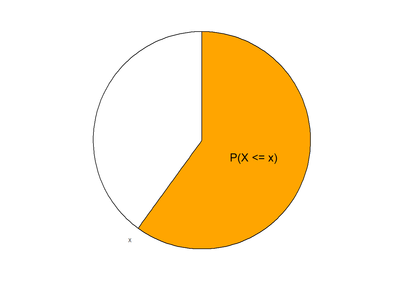
To understand a cdf, imagine a spinner for a particular distribution. Suppose a “second hand” starts at the smallest possible value (“12:00”) and sweeps clockwise around the spinner. The second hand sweeps out area as it goes; when the second hand is pointing at $x$, the area that it has swept through represents $\textrm{P}(X\le x)$. The cdf records the values of $F_X(x) = \textrm{P}(X\le x)$ as the second hand moves along and points to different values of $x$.

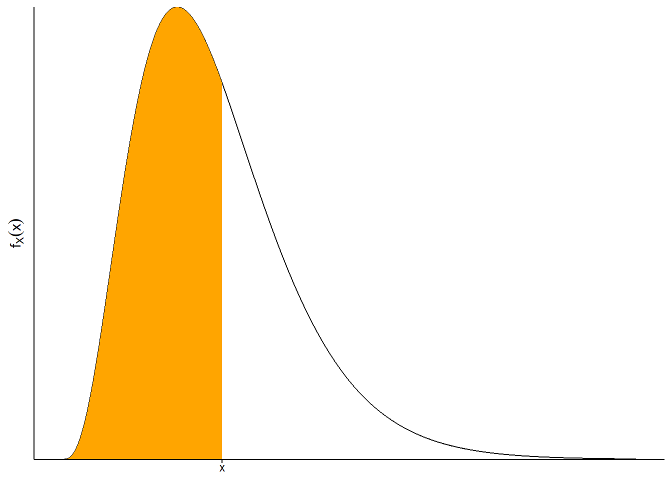
While a cdf is defined the same way for both discrete and continuous random variables, it is probably best understood in terms of continuous random variables. Remember that for a continuous random variable, $\textrm{P}(X\le x)$ is the area under the density curve over the interval $(-\infty, x]$ (remember the density might be 0 for some values in this range). Imagine plotting a density curve and adding a vertical line at $x$; $\textrm{P}(X\le x)$ is the area under the curve to left of this line. The cdf is constructed by moving the vertical line from left to right, from smaller to larger values of $x$, and recording the area under the curve to the left of the line, $F_X(x) = \textrm{P}(X\le x)$, as $x$ varies.

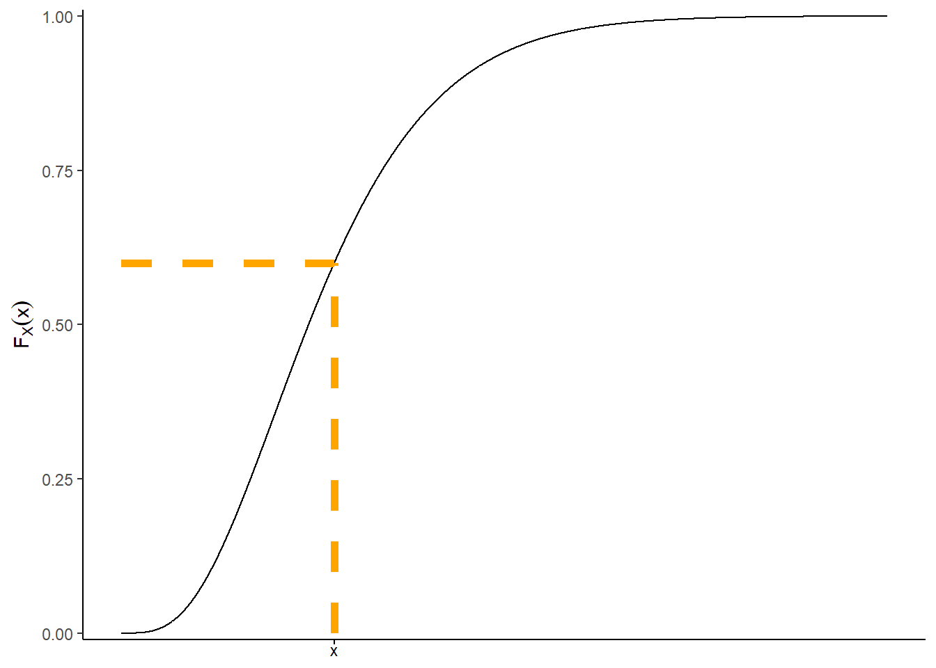
See the figure below for an illustration. The shaded area in the plot on the left represents $F_X(x)=\textrm{P}(X\le x)$, which is about 0.6 in this example. This area is represented by the $(x, F_X(x))$ point in the cdf plot in the middle. The cdf plot in the middle represents the result of recording the area in the plot on the left for all values of $x$. The plot on the right displays the spinner corresponding to the pdf on the left.

Example 4.17 Let $X$ be a random variable with the Exponential(1) distribution. Then the pdf of $f_X$ is

\[ f_X(x) = \begin{cases} e^{-x}, & x>0,\\ 0, & \text{otherwise.} \end{cases} \]

Find the cdf of $X$, and sketch a plot of it.
Evaluate and interpret $F_X(1)$, and draw a picture depicting it.
Evaluate and interpret $F_X(2)-F_X(1)$, and draw a picture depicting it.
Evaluate and interpret $F_X(2)$, and draw a picture depicting it.
Find $\textrm{P}(1 < X < 2.5)$ without integrating again.
Suppose we had been given the cdf instead of the pdf. How could we find the pdf?

Solution. to Example 4.17

Show/hide solution

$F_X(x)=0$ for $x<0$. For $x>0$ we integrate the density¹⁰⁹ \[ F_X(x) = \textrm{P}(X \le x) = \int_0^x e^{-u} du = 1 - e^{-x} \] So the cdf of $X$ is \[ F_X(x) = \begin{cases} 1 - e^{-x}, & x>0,\\ 0, & \text{otherwise.} \end{cases} \]
$F_X(1)=\textrm{P}(X\le 1) = 1-e^{-1}\approx 0.632$. This is represented by the area under the Exponential(1) density curve from 0 to 1, 63.2%.
This is represented by the area under the Exponential(1) density curve from 1 to 2, 23.3%. \[ F_X(2)- F_X(1)=\textrm{P}(X\le 2) - \textrm{P}(X \le 1) =\textrm{P}(1<X\le 2)= (1-e^{-2})-(1-e^{-1})=e^{-1}-e^{-2}\approx 0.233 \]
$F_X(2)=\textrm{P}(X\le 2) = 1-e^{-2}\approx 0.865$. This is represented by the area under the Exponential(1) density curve from 0 to 1, 63.2%+23.3% = 86.5%.
\[ \textrm{P}(1 < X < 2.5) = \textrm{P}(X\le 2.5) - \textrm{P}(X \le 1) = F_X(2.5) - F_X(1) = (1-e^{-2.5})-(1-e^{-1})=e^{-1}-e^{-2.5}\approx 0.286 \]
Since the cdf is obtained by integrating the pdf, the pdf if obtained by differentiating the cdf. Differentiate the cdf $F_X(x)=1-e^{-x},\ x>0$ with respect to its argument $x$ to obtain the pdf $f_X(x) = e^{-x},\ x>0$.

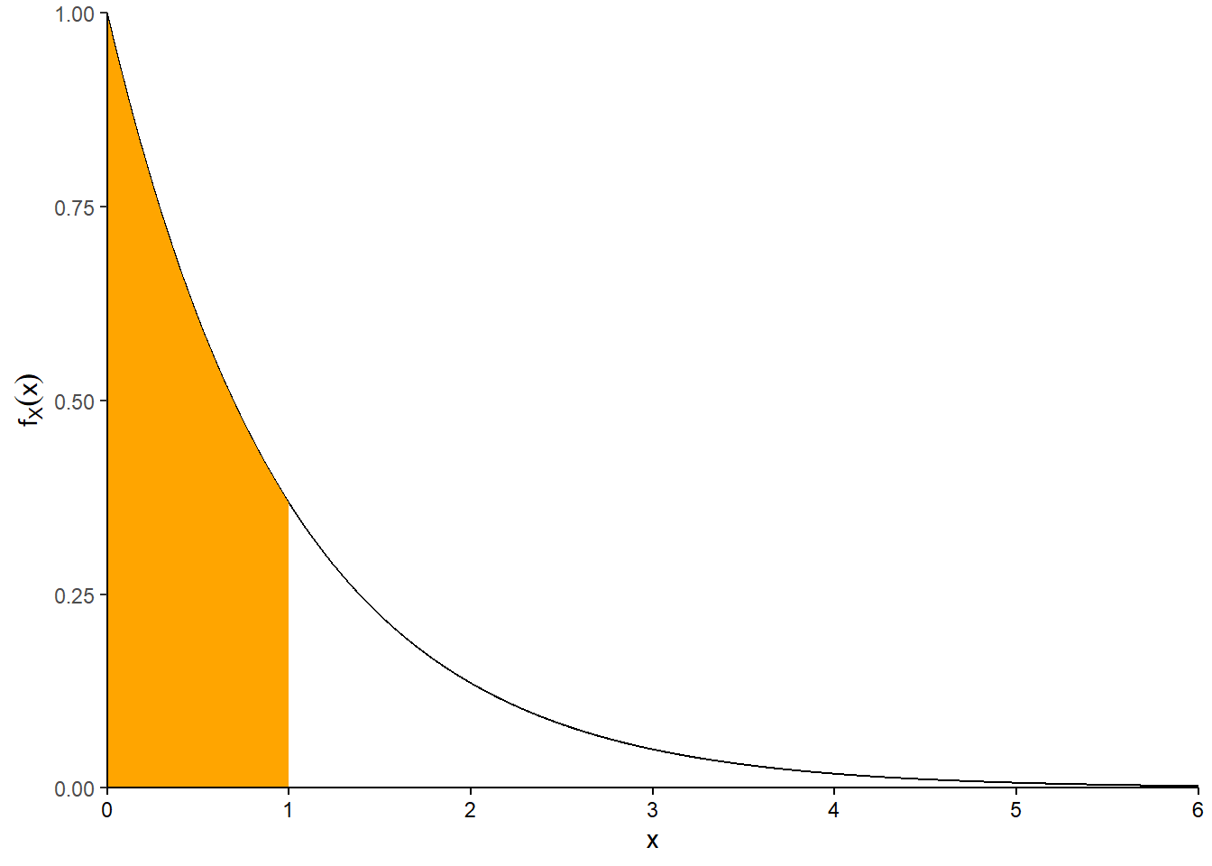
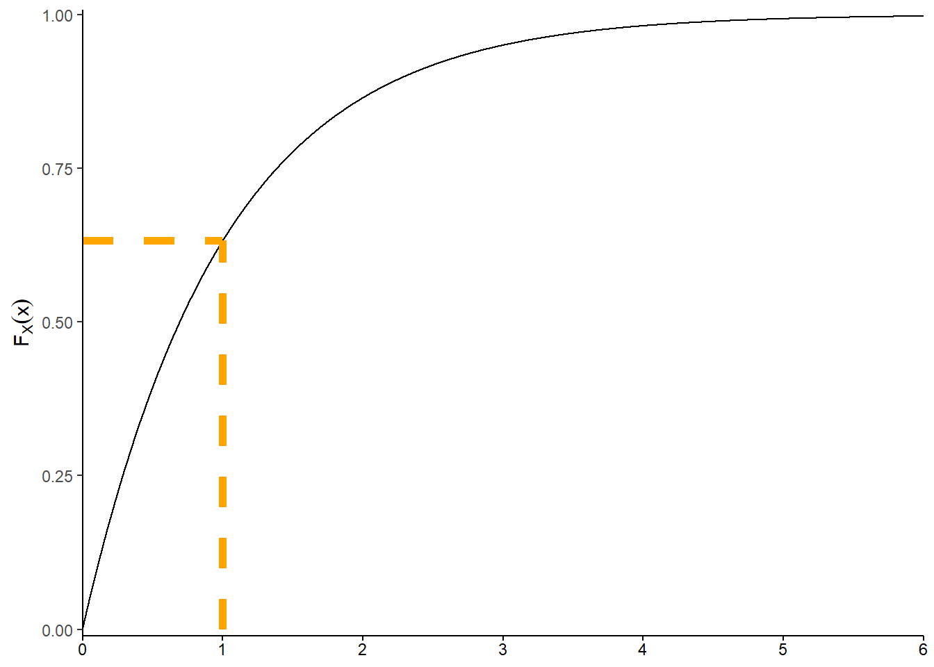
$Illustration of the pdf (left) and the cdf (right) for the Exponential(1) distribution represented by the spinner in Figure 4.13. The shaded area in the plot on the left represents $F_X(1)=\textrm{P}(X\le 1)$, which is $1-e^{-1}\approx0.632$. This area is represented by the $(1, F_X(1))$ point in the cdf plot on the right, and in the region from 0 to 1 in the spinner in Figure 4.13.$ $Illustration of the pdf (left) and the cdf (right) for the Exponential(1) distribution represented by the spinner in Figure 4.13. The shaded area in the plot on the left represents $F_X(1)=\textrm{P}(X\le 1)$, which is $1-e^{-1}\approx0.632$. This area is represented by the $(1, F_X(1))$ point in the cdf plot on the right, and in the region from 0 to 1 in the spinner in Figure 4.13.$

Figure 4.18: Illustration of the pdf (left) and the cdf (right) for the Exponential(1) distribution represented by the spinner in Figure 4.13. The shaded area in the plot on the left represents $F_X(1)=\textrm{P}(X\le 1)$, which is $1-e^{-1}\approx0.632$. This area is represented by the $(1, F_X(1))$ point in the cdf plot on the right, and in the region from 0 to 1 in the spinner in Figure 4.13.

For named distributions, we can evaluate the cdf in Symbulate using the .cdf() method.


Exponential(1).cdf(1)

## 0.6321205588285577


Exponential(1).cdf([-1, 2, 2.5])

## array([0.        , 0.86466472, 0.917915  ])

For continuous random variables, think of the cdf as a “generic integral”. Rather than integrating from scratch to find $\textrm{P}(X < 1)$, $\textrm{P}(X < 2)$, $\textrm{P}(1 < X< 2)$, etc, the integral is computed once for a generic $x$ and then evaluated to find probabilities for specific values of $x$, $F_X(1)$, $F_X(2)$, $F_X(2)-F_X(1)$, etc.

We integrate the pdf to find the cdf, and we differentiate the cdf to find the pdf. If $X$ is a continuous random variable with cdf $F_X$ then its pdf if $f_X = F'_X$.

Example 4.18 Recall Example 3.31. Let $X$ be Regina’s arrival time.

Find the cdf of $X$.
Find the pdf of $X$.

Solution. to Example 4.18

Show/hide solution

The cdf is provided by the setup: $F_X(x) = x^2, 0<x<1$. (And $F_X(x) = 0, x <0$, $F_X(x)=1, x > 1$)
Differentiate the cdf with respect to $x$. $f_X(x) = F'_X(x) = 2x$, $0<x<1$. This is the pdf in Example 4.12.

For any random variable $X$ with cdf $F_X$ \[ F_X(b) - F_X(a) = \textrm{P}(a<X \le b) \] Note that whether the inequalities in the above event are strict ($<$) or not ($\le$) matters for discrete random variables, but not for continuous.

Example 4.19 Let $X$ be the number of heads in 3 flips of a fair coin.

Find the cdf of $X$ and sketch a plot of it.
Let $Y$ be the number of tails in 3 flips of a fair coin. Find the cdf of $Y$.

Solution. to Example 4.19

Show/hide solution

See Figure 4.19. $X$ takes values 0, 1, 2, 3, with respective probabilities 1/8, 3/8, 3/8, 1/8. We sum these probabilities to find the cdf. For example, $F_X(0) = \textrm{P}(X\le 0) = 1/8$, $F_X(1)=\textrm{P}(X\le 1) = \textrm{P}(X=0) + \textrm{P}(X=1) = 1/8+3/8 = 0.5$. Remember that $x$ is defined for any value of $x$, for example $F_X(1.5) = \textrm{P}(X\le 1.5)= \textrm{P}(X=0) + \textrm{P}(X=1)=0.5$. The cdf is a step function, which is flat for impossible values of $x$ and jumps at possible values $x$ with the jump size at $x$ equal to the value of the pmf at $x$. \[ F_X(x) = \begin{cases} 0, & x<0,\\ 1/8, & 0\le x<1,\\ 4/8, & 1\le x<2,\\ 7/8, & 2\le x<3,\\ 1, & x\ge 3. \end{cases} \]
The cdf describes a distribution. Since $X$ and $Y$ have the same distribution, they will have the same cdf. The only difference would be labeling; we would call the cdf of $Y$, $F_Y$, and the argument of this function would typically (but not necessarily) be denoted $y$.

$Illustration of the pmf (left) and the cdf (right) of $X$, the number of heads in 3 flips of a fair coin. The possible values of $X$ are 0, 1, 2, 3. The pmf on the left displays the probabilities of these values, $p_X(x) = \textrm{P}(X=x)$. The cdf on the right displays $F_X(x)=\textrm{P}(X\le x)$. The cdf is flat between possible values, and jumps at the possible values, with the jumps sizes given by the pmf. (The corresponding distribution is the “Binomial(3, 0.5)” distribution.)$ $Illustration of the pmf (left) and the cdf (right) of $X$, the number of heads in 3 flips of a fair coin. The possible values of $X$ are 0, 1, 2, 3. The pmf on the left displays the probabilities of these values, $p_X(x) = \textrm{P}(X=x)$. The cdf on the right displays $F_X(x)=\textrm{P}(X\le x)$. The cdf is flat between possible values, and jumps at the possible values, with the jumps sizes given by the pmf. (The corresponding distribution is the “Binomial(3, 0.5)” distribution.)$

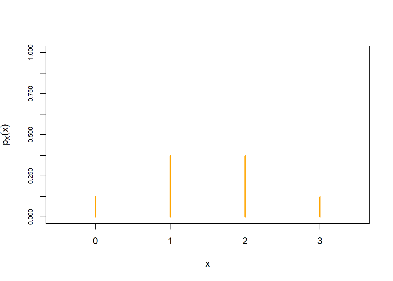
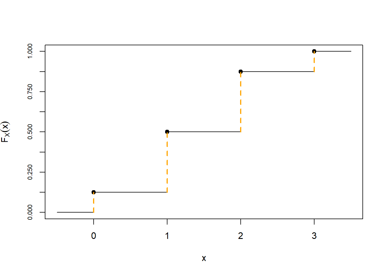
Figure 4.19: Illustration of the pmf (left) and the cdf (right) of $X$, the number of heads in 3 flips of a fair coin. The possible values of $X$ are 0, 1, 2, 3. The pmf on the left displays the probabilities of these values, $p_X(x) = \textrm{P}(X=x)$. The cdf on the right displays $F_X(x)=\textrm{P}(X\le x)$. The cdf is flat between possible values, and jumps at the possible values, with the jumps sizes given by the pmf. (The corresponding distribution is the “Binomial(3, 0.5)” distribution.)


Binomial(3, 0.5).cdf(2)

## 0.875


Binomial(3, 0.5).cdf([-1, 0, 0.5, 0.99, 1, 1.1, 2.4, 2.9, 3, 3.1, 3.9999, 4, 10])

## array([0.   , 0.125, 0.125, 0.125, 0.5  , 0.5  , 0.875, 0.875, 1.   ,
##        1.   , 1.   , 1.   , 1.   ])

A few properties of cdfs

A cdf is defined for all values of $x$, regardless if $x$ is a possible value of the RV.
A cdf is a non-decreasing function¹¹⁰: if $x_1 \le x_2$ then $F_X(x_1)\le F_X(x_2)$.
A cdf approaches 0 as the input approaches $-\infty$: $\lim_{x\to-\infty}F_X(x) = 0$
A cdf approaches 1 as the input approaches $\infty$: $\lim_{x\to\infty}F_X(x) = 1$
The cdf of a discrete random variable is a step function.
- The steps occur at the possible values of the random variable.
- The height of a particular step corresponds to the probability of that value, given by the pmf.
The cdf of a continuous random variable is a continuous function.
- The cdf of a continuous random variable is obtained by integrating the pdf, so
- The pdf of a continuous random variable is obtained by differentiating the cdf \[ F_X' = f_X \qquad \text{if $X$ is continuous} \]
For any random variable $X$ with cdf $F_X$ \[ F_X(b) - F_X(a) = \textrm{P}(a<X \le b) \] Whether the inequalities in the above event are strict ($<$) or not ($\le$) matters for discrete random variables, but not for continuous.

One advantage to using cdfs is that they are defined the same way ($F_X(x) = \textrm{P}(X\le x)$) for both continuous and discrete random variables. So results stated in terms of cdfs apply for both discrete and continuous random variables. This is a little more convenient than having two versions of every definition/result/proof: a statement for discrete RVs in terms of pmfs and a separate statement for continuous RVs in terms of pdfs. The following definition is an example.

Definition 4.8 Random variables $X$ and $Y$ have the same distribution if their cdfs are the same, that is, if $F_X(u) = F_Y(u)$ for all¹¹¹ $u\in\mathbb{R}$.

That is, two random variables have the same distribution if all the percentiles are the same. While we generally think of two discrete random variables having the same distribution if they have the same pmf, and two continuous random variables having the same distribution if they have the same pdf, the above definition provides a consistent criteria for any two random variables to have the same distribution, regardless of type.

Example 4.20 Randomly select a car insurance policy and let $X$ be the amount of claims in a year for the policy, measured in thousands of dollars, which could be 0 if the policy has no claims. Suppose the cdf of $X$ is \[ F_X(x) = 1-0.06e^{-x / 4.3}, \quad x\ge 0 \]

Compute and interpret $\textrm{P}(X \le 2)$.
Compute and interpret $\textrm{P}(X > 2)$.
Compute $\textrm{P}(X \le -0.001)$
Compute $\textrm{P}(X \le 0)$.
Compute and interpret $\textrm{P}(X = 0)$. Be careful! (Hint: see the two previous parts. Draw the cdf, starting from $x < 0$ and see what happens at $x = 0$.)
Compute and interpret $\textrm{P}(X > 0)$. Be careful!
Compute and interpret $\textrm{P}(0 < X \le 2)$. Be careful!
Is $X$ discrete, continuous, or neither? Explain.
Compute and interpret $\textrm{P}(X > 2 | X > 0)$.
Find $\textrm{P}(X > x | X > 0)$ for $x > 0$.
Identify by name the conditional distribution of $X$ given $X>0$, including the values of relevant parameters.
Describe a “two-stage” process for simulating values of $X$.

Solution. to Example 4.20

Show/hide solution

$\textrm{P}(X \le 2) = F_X(2) = 1 - 0.06e^{-2/4.3} = 0.962$. About 96.2% of policies have claims no larger than 2 thousand dollars.
$\textrm{P}(X > 2) = 1 - \textrm{P}(X \le 2) = 1 - F_X(2) = 0.06e^{-2/4.3} = 0.038$. About 3.8% of policies have claims greater than 2 thousand dollars.
$\textrm{P}(X \le -0.001) = F_X(-0.001) = 0$
$\textrm{P}(X \le 0) = F_X(0) = 1 - 0.06e^{-0/4.3} = 1 - 0.06 = 0.94$.
$F(x) = 0$ for all $x<0$ so $\textrm{P}(X < 0) = 0$. But $\textrm{P}(X\le 0) = 0.94.$ So $\textrm{P}(X = 0) = \textrm{P}(X\le 0) - \textrm{P}(X < 0) = 0.94 - 0$. About 94% of policies have no claims.
$\textrm{P}(X> 0) = 1 - \textrm{P}(X \le 0) = 1 - F_X(0) = 0.06e^{-0/4.3} = 0.06.$ About 6% of policies have non-zero claims.
$\textrm{P}(0 < X \le 2) = F_X(2) - F_X(0) = (1-0.06e^{-2/4.3}) - (1-0.06e^{-0/4.3}) = 0.962 - 0.94 = 0.022$. About 2.2% of policies have non-zero claims less than 2 thousand dollars.
$X$ is neither discrete or continuous; it’s a mixture of both. We see that $\textrm{P}(X=0) > 0$, so $X$ is not continuous. But also any value $X \ge 0$ is possible, so it’s not discrete either. Here $X$ is mixed discrete and continuous. 94% of policies have no claims, so there is a spike at 0. But among the policies that do have claims, the amounts follow a continuous distribution (here it’s Exponential). If you plot the cdf, there is a jump at $x = 0$ (from 0 to 0.94) but then it is continuous for $x>0$.
Use the definition of conditional probability \[ \textrm{P}(X > 2 | X > 0) = \frac{\textrm{P}(X> 2, X>0)}{\textrm{P}(X > 0)} = \frac{\textrm{P}(X> 2)}{\textrm{P}(X > 0)} = \frac{0.06e^{-2 / 4.3}}{0.06} = e^{-2 / 4.3} = 0.628. \] About 62.8% of policies that have non-zero claims have claims greater than 2 thousand dollars.
Similar to the previous part for a generic $x>0$ \[ \textrm{P}(X > x | X > 0) = \frac{\textrm{P}(X> x, X>0)}{\textrm{P}(X > 0)} = \frac{\textrm{P}(X> x)}{\textrm{P}(X > 0)} = \frac{0.06e^{-x / 4.3}}{0.06} = e^{-x / 4.3}. \]
The key is to recognize that $e^{-x/4.3}$ is the one minus the cdf of the Exponential(1/4.3) distribution. Therefore, the conditional cdf of $X$ given $X>0$ is the cdf of the Exponential(1/4.3) distribution. That is, the conditional distribution of $X$ given $X>0$ is the Exponential(1/4.3) distribution, with rate parameter 1/4.3 and long run average 4.3 thousand dollars. Among policies with non-zero claims, the distribution of claim amounts follows an Exponential(1/4.3) distribution. Among policies with non-zero claims, the average claim amount is 4.3 thousand dollars.
First, simulate whether or not the policy has a non-zero claim: construct a spinner than lands on “no claim” with probability 0.94 and “claim” with probability 0.06. If this spinner lands on “no claim” set $X = 0$. Otherwise, simulate a value from an Exponential(1/4.3) distribution — for example, by simulating a value from the Exponential(1) spinner and multiplying the result by 4.3 — and let $X$ be the simulated value.

The random variable in the previous example is a mixed discrete and continuous random variable. The cdf has both discrete (jumps) and continuous features.

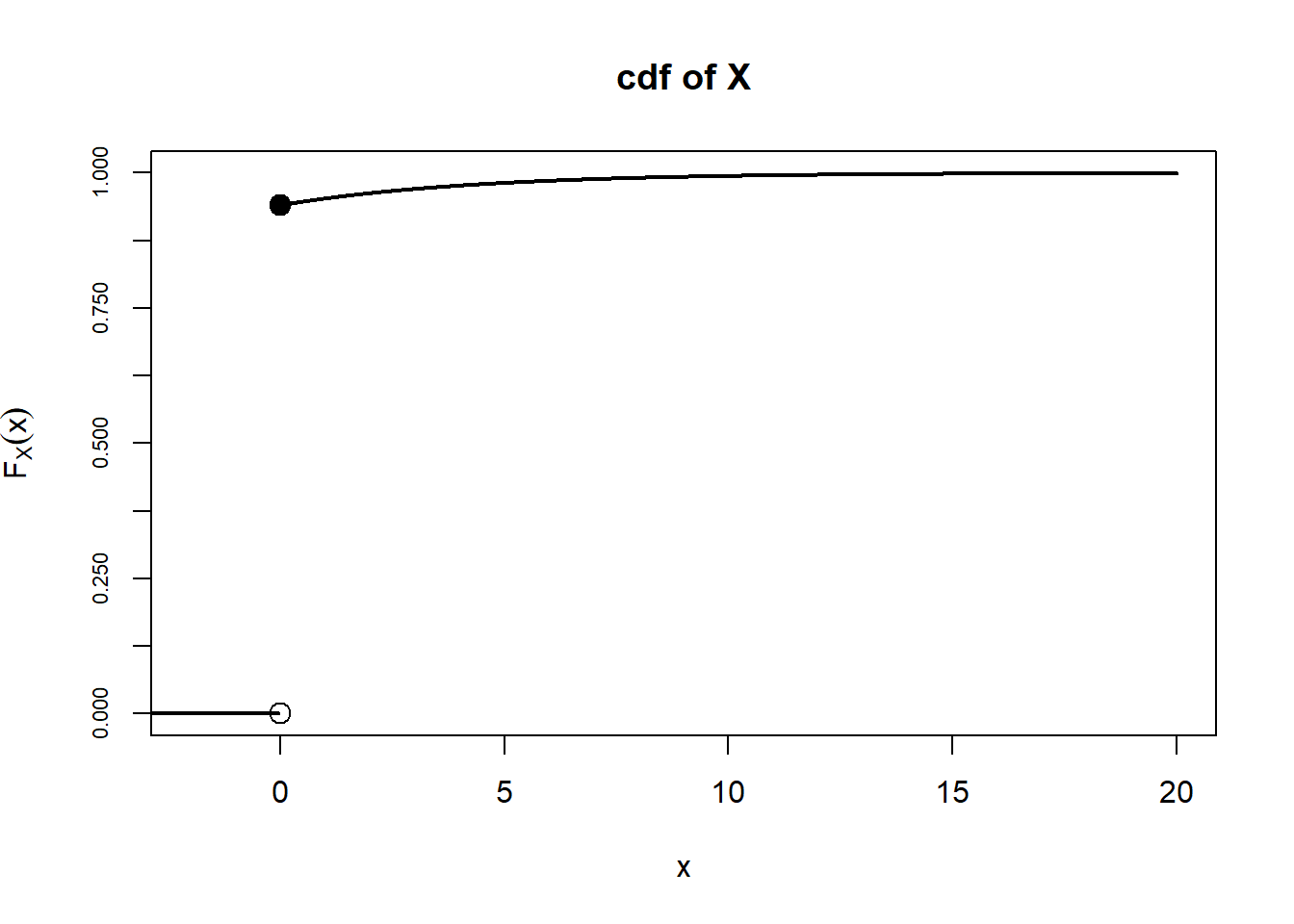
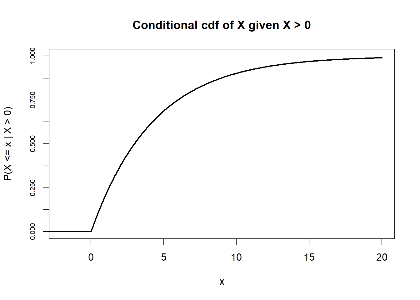
$Illustration of the cdf of $X$ (left) and the conditional cdf of $X$ given $X>0$ (right) in Example 4.20.$ $Illustration of the cdf of $X$ (left) and the conditional cdf of $X$ given $X>0$ (right) in Example 4.20.$

Figure 4.20: Illustration of the cdf of $X$ (left) and the conditional cdf of $X$ given $X>0$ (right) in Example 4.20.

The code below implements the two-stage method for simulating values of $X$ discussed in the example. $I$ indicates if there is a claim ($I=1$) or not $(I=0)$. $Y$ is the output of the Exponential(1/4.3) spinner. Defining $X = IY$ reflects that if $I= 0$ then $X=0$, otherwise $X = Y$.

I, Y = RV(BoxModel([0, 1], probs = [0.94, 0.06]) * Exponential(rate = 1 / 4.3))

X = I * Y

x = X.sim(10000)

x

Index	Result
0	0.0
1	0.0
2	0.0
3	0.0
4	0.0
5	0.0
6	0.0
7	0.0
8	0.0
...	...
9999	0.0

The histogram is obscured by the large proportion of zeros. For mixed discrete and continuous random variables like this, it is often better to summarize the discrete and continuous parts separately.

x.plot()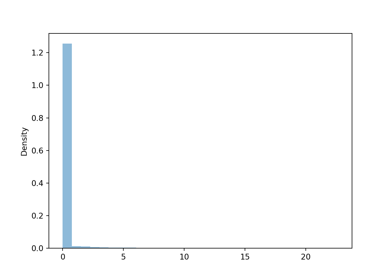

x.count_eq(0) / x.count()

## 0.9388

x.count_gt(2) / x.count()

## 0.0378

x.mean()

## 0.2441275379871232

Now we condition on policies that have non-zero claims. Among the policies with non-zero claims, the claim amounts follow an Exponential(1/4.3) distribution.

x_given_not0 = (X | (X > 0) ).sim(10000)

x_given_not0

Index	Result
0	1.4612610509504205
1	3.567580796919767
2	1.4888183356554903
3	10.461979720752733
4	0.3155926531346989
5	0.09086595808906088
6	1.5942529481519125
7	0.9984177709935759
8	6.7574305265451615
...	...
9999	1.3695176283937025

x_given_not0.plot() # plot the simulated values

Exponential(rate = 1 / 4.3).plot() # plot the theoretical pdf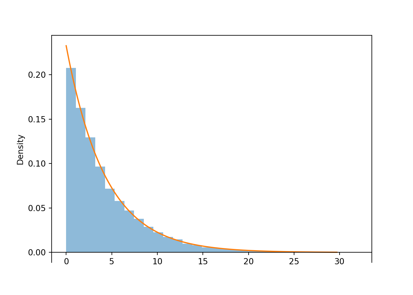

x_given_not0.count_gt(2) / x_given_not0.count()

## 0.6265

x_given_not0.mean()

## 4.262813857819792

Here $x$ represents a particular value of interest, so we use a different dummy variable, $u$, in the integrand.↩︎
This follows from the subset rule, since if $x_1\le x_2$ then $\{X\le x_1\}\subseteq\{X\le x_2\}$↩︎
Note that $u$ just represents a dummy variable, the argument of the two functions. While we generally think of $x$ as the argument of $F_X$, that is just a convenient labeling. Here we are checking for equality of two functions, so we need to use the same input for both. That is, something like “$F_X(x) = F_Y(y)$” makes no sense because $x$ and $y$ represent different inputs.↩︎