1.4 Proportional reasoning and tables of counts
It is often helpful to think of probabilities as percentages or proportions. Furthermore, when working with multiple percentages, it is also helpful to construct hypothetical tables of counts.
Example 1.9 Are Americans in favor of free tuition at public colleges and universities? Suppose that10
- 83% of Democrats are in favor of free tuition
- 60% of Independents are in favor of free tuition
- 39% of Republicans are in favor of free tuition
Also suppose that11
- 32% of Americans are Democrats
- 42% of Americans are Independents
- 26% of Americans are Republicans
We’ll use this information to investigate the following questions, as well as a few others.
- What percentage of Americans are in favor of free college tuition?
- What percentage of Americans who are in favor of free college tuition are Democrats?
Donny Don’t says the answer to the question “what percentage of Americans who are in favor of free college tuition are Democrats” is 83%. Explain why Donny is wrong without doing any calculations.
For the remaining parts, consider a hypothetical group of 10000 Americans and assume the percentages provided apply to this group. How many people in the group are Democrats?
How many Americans in the group are Democrats who are in favor of free college tuition?
Fill in the counts in each of the cells of the following table.
Democrat Independent Republican Total In favor of free tuition Not in favor of free tuition Total 10000 What percentage of Americans in this group who are in favor of free college tuition are Democrats? (Answer with both an unreduced fraction and a percent.)
Suppose we had started with a hypothetical group of 100,000 Americans. How would the table of counts change? Would the answer to the previous part change?
Now answer the original question: What percentage of Americans who are in favor of free college tuition are Democrats?
What percentage of Americans who are Democrats are in favor of free college tuition? (Answer with both an unreduced fraction and a percent.)
What percentage of Americans are Democrats in favor of free college tuition? (Answer with both an unreduced fraction and a percent.)
Compare the unreduced fractions for the previous three parts. What is the same? What is different?
What percentage of Americans are in favor of free college tuition?
Suppose that we were only told that 61.9% of Americans overall support free tuition, and that we not given the values 83%, 60%, 39%. Would we be able to complete the two-way table?
Solution. to Example 1.9
Show/hide solution
Donny is confusing two different percentages, which refer to two different groups.
- 83% of Democrats are in favor of free college tuition. This percentage applies to Democrats; among Democrats what percentage are in favor of free college tuition?
- What we want is the percent of Americans in favor of free tuition who are Democrats. This percentage applies to Americans in favor of free tuition; among Americans in favor of free tuition what percentage are Democrats?
Of the 10000 Americans, 32%, that is 3200, are Democrats. (\(0.32 \times 10000 = 3200\))
Out of the 3200 Democrats, 83%, that is 2656 are in favor of free tuition. (\(3200 \times 0.83 = 2656\))
We fill in the total for each party first. Then we use the percentages to determine the number who are in favor of free tuition within each party. For example, 60% of the 4200 Independents are in favor of free tuition. (\(4200 \times 0.6 = 2520\))
Democrat Independent Republican Total In favor of free tuition 2656 2520 1014 6190 Not in favor of free tuition 544 1680 1586 3810 Total 3200 4200 2600 10000 Out of 6190 Americans in this group who are in favor of free college tuition, 2656 are Democrats. Since \(\frac{2656}{6190}\approx 0.43\), about 43% of Americans in this group who are in favor of free college tuition are Democrats.
If we had started with a hypothetical group of 100,000 Americans then the count in every cell in the table would be 10 times greater. However, ratios and percentages would still be the same. The answer to the previous part would not change; it would still be \(\frac{26560}{61900} =\frac{2656}{6190}\approx 0.43\).
Now we are interested in Americans in general rather than the 10000 Americans in our hypothetical group. But as the previous part illustrates, the relative percentages will be the same regardless of the size of the group. So we can say that 43% of Americans who are in favor of free college tuition are Democrats.
We were provided the percentage of Americans who are Democrats that are in favor of free college tuition, 83%, or from the table, \(\frac{2656}{3200}\). Pay careful attention to the difference in wording between this part and the previous one.
Out of 10000 Americans, 2656 are Democrats in favor of free college tuition, so \(\frac{2656}{10000}= 26.56\%\) of Americans are Democrats in favor of free college tuition.
There are subtle but important differences in wording between the percentages of interest in the previous three parts. Note that the numerator is the same in each part: 2656, the number of Americans in the group who are both Democrats and in favor of free tuition. But the denominators are different, each corresponding to a different reference group
- the percentage of Americans who favor free tuition… (denominator of 6190)
- the percentage of Americans who are Democrats… (denominator of 3200)
- the percentage of Americans… (denominator of 10000)
Out of 10000 Americans, 6190 are in favor of free college tuition, so 61.9% of Americans are in favor of free college tuition.
Even if 61.9% of Americans overall support free tuition, it would not be safe to assume that 61.9% of Democrats support, 61.9% of Independent support, and 61.9% of Republicans support. We would expect support to vary by party, but without such information we would not be able to complete the two-way table.
Two-way tables (a.k.a., contingency tables) of counts are a useful tool for probability problems dealing with two events. For the purposes of constructing the table and computing related probabilities, any value can be used for the hypothetical12 total count13.
When dealing with percentages (or proportions or probabilities) be sure to ask “percent of what?” Thinking in fraction terms, be careful to identify the correct reference group which corresponds to the denominator.
Example 1.10 Which of the following is larger - 1 or 2?
- The probability that a randomly selected man who is greater than six feet tall plays in the NBA.
- The probability that a randomly selected man who plays in the NBA is greater than six feet tall.
Solution. to Example 1.10
Show/hide solution
The probability in (2) is much larger. Think in terms of fractions. The corresponding fractions would have the same numerator — number of men who are both greater than six feet tall and play in the NBA — but vastly different denominators.
\[\begin{align*} (1): & \quad \frac{\text{number of men who are greater than six feet tall and play in the NBA}}{\text{number of men who are greater than six feet tall}}\\ (2): & \quad \frac{\text{number of men who are greater than six feet tall and play in the NBA}}{\text{number of men who play in the NBA}} \end{align*}\]
- There are over a billion men in the world who are greater than six feet tall, only a few hundred of whom play in the NBA. The probability that a randomly selected man who is greater than six feet tall plays in the NBA is pretty close to 0.
- There only a few hundred men who play in the NBA, almost all of whom are greater than six feet tall. The probability that a randomly selected man who plays in the NBA is greater than six feet tall is pretty close to 1.
In Example 1.9, we needed the information about support for free tuition within in each party to fill in the table. That is, it was not enough to know that 61.9% of Americans overall support free tuition. In general, knowing probabilities of individual events alone is not enough to determine probabilities of combinations of them.
Example 1.11 Suppose that 47% of American adults14 have a pet dog and 25% have a pet cat.
- Donny Don’t says that 72% (which is 47% + 25%) of American adults have a pet dog or a pet cat. Is that necessarily true? If not, is it even possible (in principle anyway) for this to be true? Under what circumstance (however unrealistic) would this be true? Construct a corresponding two-way table.
- Given only the information provided, what is the smallest possible percentage of American who adults have a pet dog or a pet cat. Under what circumstance (however unrealistic) would this be true? Construct a corresponding two-way table.
- Donny Don’t says that 11.75% (which is 47% \(\times\) 25%) of Americans have both a pet dog and a pet cat. Explain to Donny why that’s not necessarily true. Without further information, what can you say about the percent of American adults who have both a pet dog and a pet cat?
- Suppose that 14% of American adults have both a pet dog and a pet cat. What is the percentage of American adults who have a pet dog or a pet cat? Construct a corresponding two-way table. Use your table to show Donny how to correct his error from part 1.
- What percentage of American adults who have a pet dog also have a pet cat? Is it 25%?
- What percentage of American adults who do not have a pet dog have a pet cat? Is this the same value as in the previous part?
Solution. to Example 1.11
Show/hide solution
Donny’s conclusion isn’t necessarily true because some people have both a pet dog and a pet cat. By adding 47% and 25%, Donny has double-counted the people who have both a dog and a cat. It’s theoretically possible that 72% have a pet dog or a pet cat, but this would only be true if absolutely no Americans have both a pet dog and a pet cat (which is obviously not realistic). The two-way table corresponding to Donny’s claim is
Have dog No dog Total Have cat 0 25 25 No cat 47 28 75 Total 47 53 100 The situation in the previous part corresponds to the largest possible value, 72%, which occurs when the percentage who have both a dog and cat is as small as possible (0%). Now we consider the reverse situation. The largest possible percentage who have both a dog and cat is 25%. Theoretically this is possible, but it would only occur if every person who has a cat also has a dog, which isn’t realistic. The two-way table would be
Have dog No dog Total Have cat 25 0 25 No cat 22 53 75 Total 47 53 100 Thus the smallest possible percentage of American adults who have a pet dog or a pet cat is 47%.
In the first two parts of this problem we have provided two theoretically possible (though unrealistic) scenarios of how Donny’s claim would be false: if no Americans who have a pet dog have a pet cat, and if 100% of Americans who have a pet dog also have a pet cat. Donny’s claim would be true if exactly 25% of American adults who have a pet dog also have a pet cat. (Equivalently, his claim would be true if exactly 47% of American adults who have a pet cat also have a pet dog.) But all we are given so far is that 25% of American adults in general have a pet cat. The likelihood of having a pet cat might change based on whether or not the adult has a dog. We would need more information about the relationship between pet dog and pet cat ownership before we could determine what percentage of American adults have both. Without further information, all we can say is that between 0% and 25% of Americans have both a pet dog and a pet cat.
If 14% of American adults have both a dog and a cat the two-way table is
Have dog No dog Total Have cat 14 11 25 No cat 33 42 75 Total 47 53 100 Therefore 58% of American adults have a pet dog or a pet cat (58 = 14 + 11 + 33). In other words, 42% of of American adults have neither a pet dog nor a pet cat. We can show Donny that adding 47% and 25% double counts the 14% who have both. Donny should have subtracted 14% to correct for the double-counting: 58 = 47 + 25 - 14.
Out of the 47 (hypothetical) adults who have a pet dog, 14 also have a pet cat, and \(\frac{14}{47} = 0.298\). So 29.8% of American adults who have a pet dog also have a pet cat. American adults who have a pet dog are a little more likely than American adults in general to have a pet cat.
Out of the 53 (hypothetical) people who do not have a pet dog, 11 have a pet cat, and \(\frac{11}{53} = 0.208\). So 20.8% of American adults who do not have a pet dog have a pet cat. This is not the same value in the previous part. People with pet dogs are more likely than people without pet dogs to have a pet cat.
Example 1.12 A woman’s chances of giving birth to a child with Down syndrome increase with age. The CDC estimates15 that a woman in her mid-to-late 30s has a risk of conceiving a child with Down syndrome of about 1 in 250. A nuchal translucency (NT) scan, which involves a blood draw from the mother and an ultrasound, is often performed around the 13th week of pregnancy to test for the presence of Down syndrome (among other things). If the baby has Down syndrome, the probability that the test is positive is about 0.9. However, when the baby does not have Down syndrome, there is still a probability that the test returns a (false) positive of about16 0.05. Suppose that the NT test for a pregnant woman in her mid-to-late 30s comes back positive for Down syndrome. What is the probability that the baby actually has Down syndrome?
- Before proceeding, make a guess for the probability in question. \[ \text{0-20\%} \qquad \text{20-40\%} \qquad \text{40-60\%} \qquad \text{60-80\%} \qquad \text{80-100\%} \]
- Donny Don’t says: 0.90 and 0.05 should add up to 1, so there must be a typo in the problem. Do you agree?
- Considering a hypothetical population of babies (of pregnant women in this demographic), express the probabilities as percents in context.
- Construct a hypothetical two-way table of counts.
- Use the table to find the probability in question.
- The probability in the previous part might seem very low to you. Explain why the probability is so low.
- Compare the probability of having Down Syndrome before and after the positive test. How much more likely is a baby who tests positive to have Down Syndrome than a baby for whom no information about the test is available?
Solution. to Example 1.12
Show/hide solution
We don’t know what you guessed, but from experience many people guess 80-100%. Afterall, the test is correct for most of the babies who have Down Syndrome, and also correct for the most of the babies who do not have Down Syndrome, so it seems like the test is correct most of the time. But this argument ignores one important piece of information that has a huge impact on the results: most babies do not have Down Syndrome.
No, these probabilities apply to different groups: 0.9 to babies with Down Syndrome, and 0.05 to babies without Down Syndrome. Donny is using the complement rule incorrectly. For example, if 0.9 is the probability that a baby with Down Syndrome tests positive, then 0.1 is the probability that a baby with Down Syndrome does not test positive; both probabilities apply to babies with Down Syndrome, and each baby with Down Syndrome either tests positive or not.
Considering a hypothetical population of babies (of pregnant women in this demographic):
- 0.4% of babies have Down Syndrome
- 90% of babies with Down Syndrome test positive
- 5% of babies without Down Syndrome test positive
- We want to find the percentage of babies who test positive that have Down Syndrome.
Assuming 10000 babies (of pregnant women in this demographic)
Has Down Syndrome Does Not have Down Sydrome Total Tests positive 36 498 534 Not test positive 4 9462 9466 Total 40 9960 10000 Among the 534 babies who test positive, 36 have Down Syndrome, so the probability that a baby who tests positive has Down Syndrome is 36/534 = 0.067.
The result says that only 6.7% of babies who test positive actually have Down Syndrome. It is true that the test is correct for most babies with Down Syndrome (36 out of 40) and incorrect only for a small proportion of babies without Down Syndrome (498 out of 9960). But since so few babies have Down Syndrome, the sheer number of false positives (498) swamps the number of true positives (36).
Prior to observing the test result, the prior probability that a baby has Down Syndrome is 0.004. The posterior probability that a baby has Down Syndrome given a positive test result is 0.067. A baby who tests positive is about 17 times (0.067/0.004) more likely to have Down Syndrome than a baby for whom the test result is not known. So while 0.067 is still small in absolute terms, the posterior probability is much larger relative to the prior probability.
Remember to ask “percentage of what”? For example, the percentage of babies who have Down syndrome that test positive is a very different quantity than the percentage of babies who test positive that have Down syndrome.
Probabilities are often conditional on information. Conditional probabilities (e.g., probability of Down Syndrome given a positive test) can be highly influenced by the original unconditional probabilities (e.g. probability of Down Syndrome), sometimes called the base rates. Don’t neglect the base rates when evaluating probabilities.
The example illustrates that when the base rate for a condition is very low and the test for the condition is less than perfect there will be a relatively high probability that a positive test is a false positive.
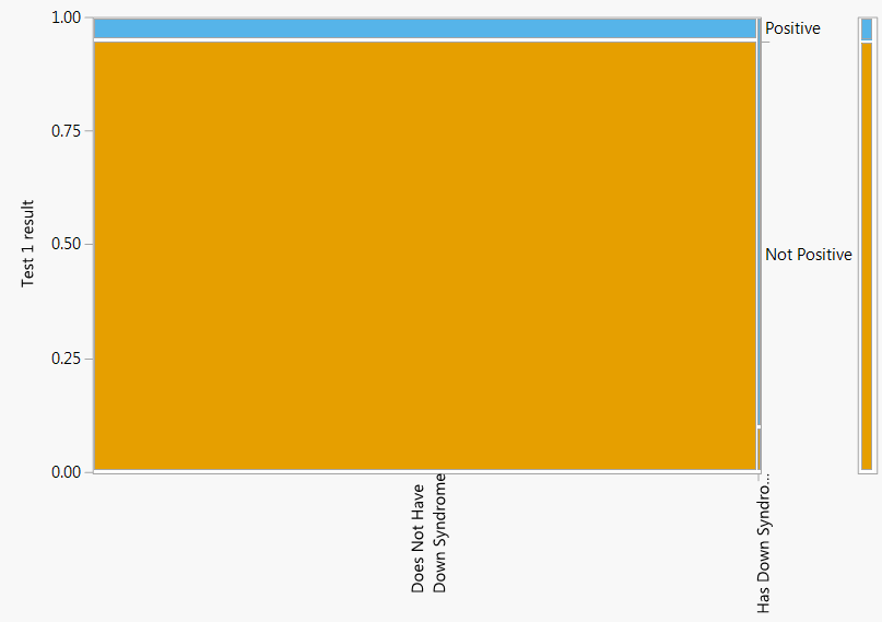
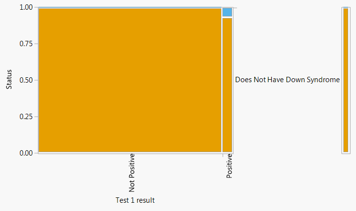
Figure 1.8: Mosaic plots for Example 1.12. The plot on the left represents conditioning on Down Syndrome status, while the plot on the right represents conditioning on test result.
1.4.1 Exercises
In each of the following, which is greater: (1) or (2)? Or are they equal? Or is there not enough information to decide?
- Surfing
- The probability that a randomly selected Californian likes to surf.
- The probability that a randomly selected American is a Californian who likes to surf
- Cal Poly alums
- The probability that a California resident is a Cal Poly alum.
- The probability that a Cal Poly alum is a California resident
- Surfing
Continuing Example 1.11
- What percentage of American adults who have a pet cat also have a pet dog?
- What percentage of American adults who do not have a pet cat have a pet cat?
- Which of these percentages is the overall percentage of American adults who have a pet dog closer to? Why do you think that is?
Continuing Example 1.11. Now suppose that 11.75% of American adults have both a pet cat and a pet dog (as Donny claimed was necessarily true). Redo Example 1.11 and the previous exercise under this assumption. What is true in this scenario that wasn’t true in Example 1.11?
Suppose that you have applied to two graduate schools, A and B. Your subjective probability of being accepted is 0.6 for school A and 0.7 for school B.
- What is the largest possible probability of being accepted by both schools? Under what scenario (however unrealistic) would this be true? Explain.
- What is the smallest possible probability of being accepted by both schools? Under what scenario (however unrealistic) would this be true? Explain.
- Explain why the probability of being accepted by both schools is not necessarily 0.42.
- For the remaining parts, suppose your subjective probability of being accepted at both schools is 0.55. If you are accepted at school A, what is your probability of also being accepted at school B?
- If you are accepted at school A, what is your probability of not being accepted at school B?
- If you are not accepted at school A, what is your probability of being accepted at school B?
- If you are accepted at school B, what is your probability of also being accepted at school A?
- If you are not accepted at school B, what is your probability of being accepted at school A?
These values are based on a study by the Pew Research Foundation conducted in January 2020.↩︎
These values are based on surveys by Gallup, but the values change somewhat over time.↩︎
Careful: we are only claiming that the total does not matter when constructing hypothetical tables. When collecting real data, the sample size matters a great deal. For example, a random sample of 1000 Americans provides a more precise estimate of the population proportion of all Americans who support free tuition than a sample of 100 Americans does. The Pew Research study was based on a sample of over 12000 Americans.↩︎
You can only run into problems if you round. Suppose we had started with a group size of 100. Then the top left cell in the table would have been 26.56. If we had rounded this to 27, our answers would change. So when dealing with a hypothetical table of counts, don’t round. If you are uncomfortable with decimal counts, just increase the size of your original group↩︎
These values are based on the 2018 General Social Survey.↩︎
Source: http://www.cdc.gov/ncbddd/birthdefects/downsyndrome/data.html↩︎
Estimates of these probabilities vary between different sources. The values in the exercise were based on https://www.ncbi.nlm.nih.gov/pubmed/17350315↩︎