4.3 Continuous random variables: Probability density functions

The continuous analog of a probability mass function (pmf) is a probability density function (pdf). However, while pmfs and pdfs play analogous roles, they are different in one fundamental way; namely, a pmf outputs probabilities directly, while a pdf does not. We have seen that a pmf of a discrete random variable can be summed to find probabilities of related events. We will see now that a pdf of a continuous random variable must be integrated to find probabilities of related events.

In Section 2.8.3 we introduced histograms to summarize simulated values of a continuous random variable. In a histogram the variable axis is chopped into intervals of equal width, and the other axis is on the density scale, so that the area of each bar represents the relative frequency of values that lie in the interval.

We have seen examples like the Normal(30, 10) distribution where the shape of the histogram can be approximated by a smooth curve. This curve represents an idealized model of what the histogram would look like if infinitely many values were simulated and the histogram bins were infinitesimally small.

Suppose we are interested in the random variable \(X = - \log(1 - U)\) where \(U\) has a Uniform(0, 1) distribution. (We will see why we might be interested in this particular transformation soon.) Here is a histogram of 10000 simulated values of \(X\).

U = RV(Uniform(0, 1))

X = -log(1 - U)

x = X.sim(10000)

x.plot()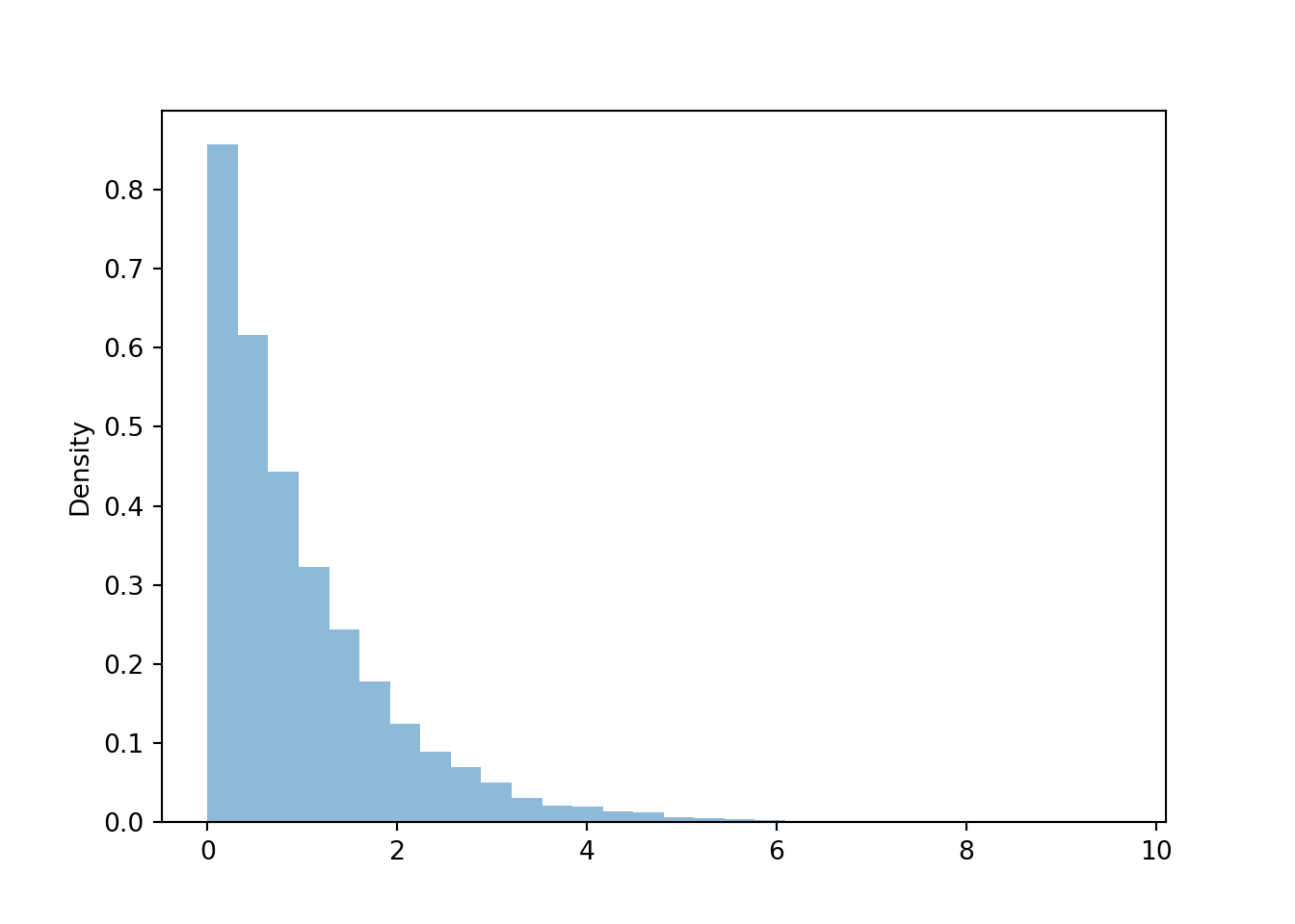

Imagine that we

• keep simulating more and more values, and
• make the histogram bin widths smaller and smaller.

Then the “chunky” histogram would get “smoother”. The following plot summarizes the results of 100,000 simulated values of \(X\) in a histogram with 1000 bins, each of width on the order of 0.01. The command Exponential(1).plot() overlays the smooth curve modeling the theoretical shape of the distribution of \(X\) (called the “Exponential(1)” distribution). This curve is an example of a pdf.

X.sim(100000).plot(bins=1000) # histogram of simulated values

Exponential(1).plot() # overlays the smooth curve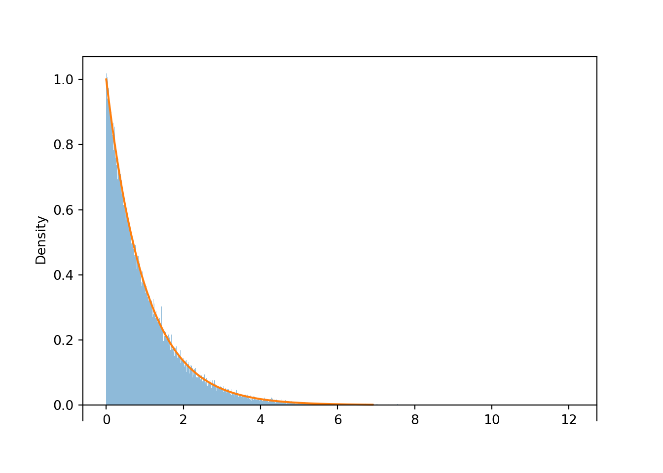

Figure 4.11: A histogram of simulated values of \(X = -\log(1-U)\), where \(U\) has a Uniform(0, 1) distribution. With many simulated values and very fine bins, the shape of the histogram is well approximated by a smooth curve, called the “Exponential(1) density”.

A pdf represents “relative likelihood” as a function of possible values of the random variable. Just as area represents relative frequency in a histogram, area under a pdf represents probability.

Definition 4.4 The probability density function (pdf) (a.k.a. density) of a continuous RV \(X\), defined on a probability space with probability measure \(\textrm{P}\), is a function \(f_X:\mathbb{R}\mapsto[0,\infty)\) which satisfies \[\begin{align*} \textrm{P}(a \le X \le b) & =\int_a^b f_X(x) dx, \qquad \text{for all } -\infty \le a \le b \le \infty \end{align*}\]

For a continuous random variable \(X\) with pdf \(f_X\), the probability that \(X\) takes a value in the interval \([a, b]\) is the area under the pdf over the region \([a,b]\).

A pdf assigns zero probability to intervals where the density is 0. A pdf is usually defined for all real values, but is often nonzero only for some subset of values, the possible values of the random variable. We often write the pdf as \[ f_X(x) = \begin{cases} \text{some function of $x$}, & \text{possible values of $x$}\\ 0, & \text{otherwise.} \end{cases} \] The “0 otherwise” part is often omitted, but be sure to specify the range of values where \(f\) is positive.

The axioms of probability imply that a valid pdf must satisfy \[\begin{align*} f_X(x) & \ge 0 \qquad \text{for all } x,\\ \int_{-\infty}^\infty f_X(x) dx & = 1 \end{align*}\]

The total area under the pdf must be 1 to represent 100% probability. Given a specific pdf, the generic bounds \((-\infty, \infty)\) in the above integral should be replaced by the range of possible values, that is, those values for which \(f_X(x)>0\).

Example 4.9 Let \(X\) be a random variable with the “Exponential(1)” distribution, illustrated by the smooth curve in Figure 4.11. Then the pdf of \(f_X\) is

\[ f_X(x) = \begin{cases} e^{-x}, & x>0,\\ 0, & \text{otherwise.} \end{cases} \]

1. Verify that \(f_X\) is a valid pdf.
2. Find \(\textrm{P}(X\le 1)\).
3. Find \(\textrm{P}(X\le 2)\).
4. Find \(\textrm{P}(1 \le X< 2.5)\).
5. Compute the 25th percentile of \(X\).
6. Compute the 50th percentile of \(X\).
7. Compute the 75th percentile of \(X\).
8. Start to construct a spinner representing the Exponential(1) distribution.

Solution. to Example 4.9

Show/hide solution

1. We need to check that the pdf integrates to 1: \(\int_0^\infty e^{-x}dx = 1\).
2. \(\textrm{P}(X\le 1) = \int_0^1 e^{-x}dx = 1-e^{-1}\approx 0.632\). See the spinner in Figure 4.13; 63.2% of the area corresponds to \([0, 1]\).
3. \(\textrm{P}(X\le 2) = \int_0^2 e^{-x}dx = 1-e^{-2}\approx 0.865\). See the spinner in Figure 4.13; 86.5% of the area corresponds to \([0, 2]\).
4. \(\textrm{P}(1 \le X< 2.5) = \int_1^{2.5} e^{-x}dx = e^{-1}-e^{-2.5}\approx 0.286\). See the illustration below.
5. We want to find \(x>0\) such that \(\textrm{P}(X \le x) =0.25\): \[ 0.25 = \textrm{P}(X \le x) = \int_0^{x} e^{-u}du = 1 - e^{-x} \] Solve to get \(x = -\log(1-0.25) = 0.288\). 25% of values of \(X\) are at most 0.288. The value 0.288 goes at 3 o’clock on the spinner axis.
6. We want to find \(x>0\) such that \(\textrm{P}(X \le x) =0.5\): \[ 0.5 = \textrm{P}(X \le x) = \int_0^{x} e^{-u}du = 1 - e^{-x} \] Solve to get \(x = -\log(1-0.5) = 0.693\). 50% of values of \(X\) are at most 0.693. The value 0.693 goes at 6 o’clock on the spinner axis.
7. We want to find \(x>0\) such that \(\textrm{P}(X \le x) =0.75\): \[ 0.75 = \textrm{P}(X \le x) = \int_0^{x} e^{-u}du = 1 - e^{-x} \] Solve to get \(x = -\log(1-0.75) = 1.386\). 75% of values of \(X\) are at most 1.386. The value 1.386 goes at 9 o’clock on the spinner axis.
8. See the spinner in Figure 4.13. It’s the same spinner on both sides, with different values highlighted. Notice that intervals near 0 are stretched out, while intervals away from 0 are shrunk.

The shaded area under the curve below represents \(\textrm{P}(1<X<2.5)\).

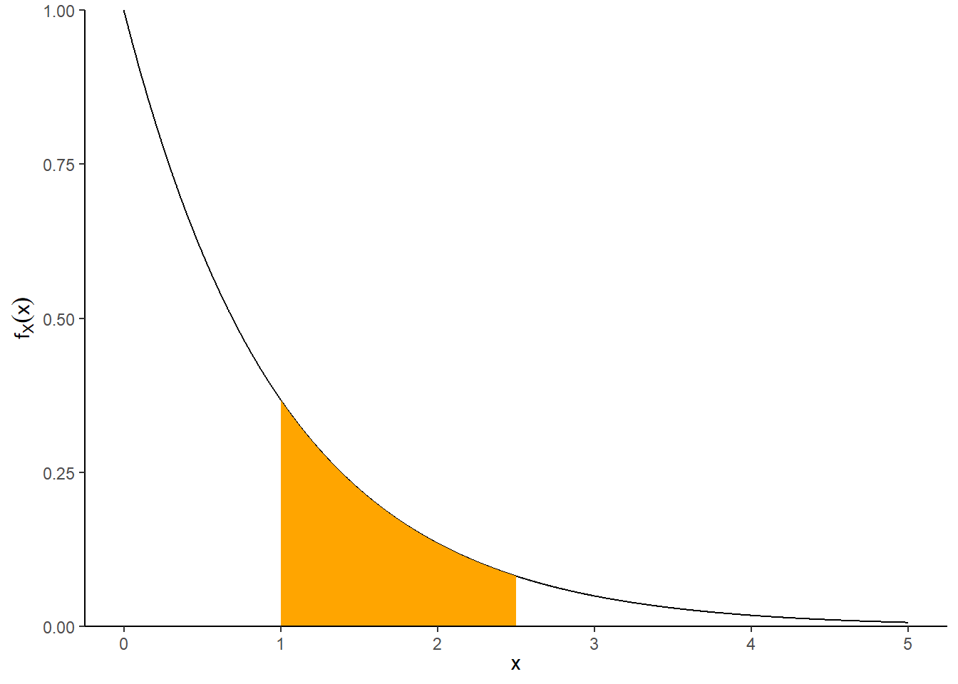
Figure 4.12: Illustration of \(\textrm{P}(1<X<2.5)\) for \(X\) with an Exponential(1) distribution.

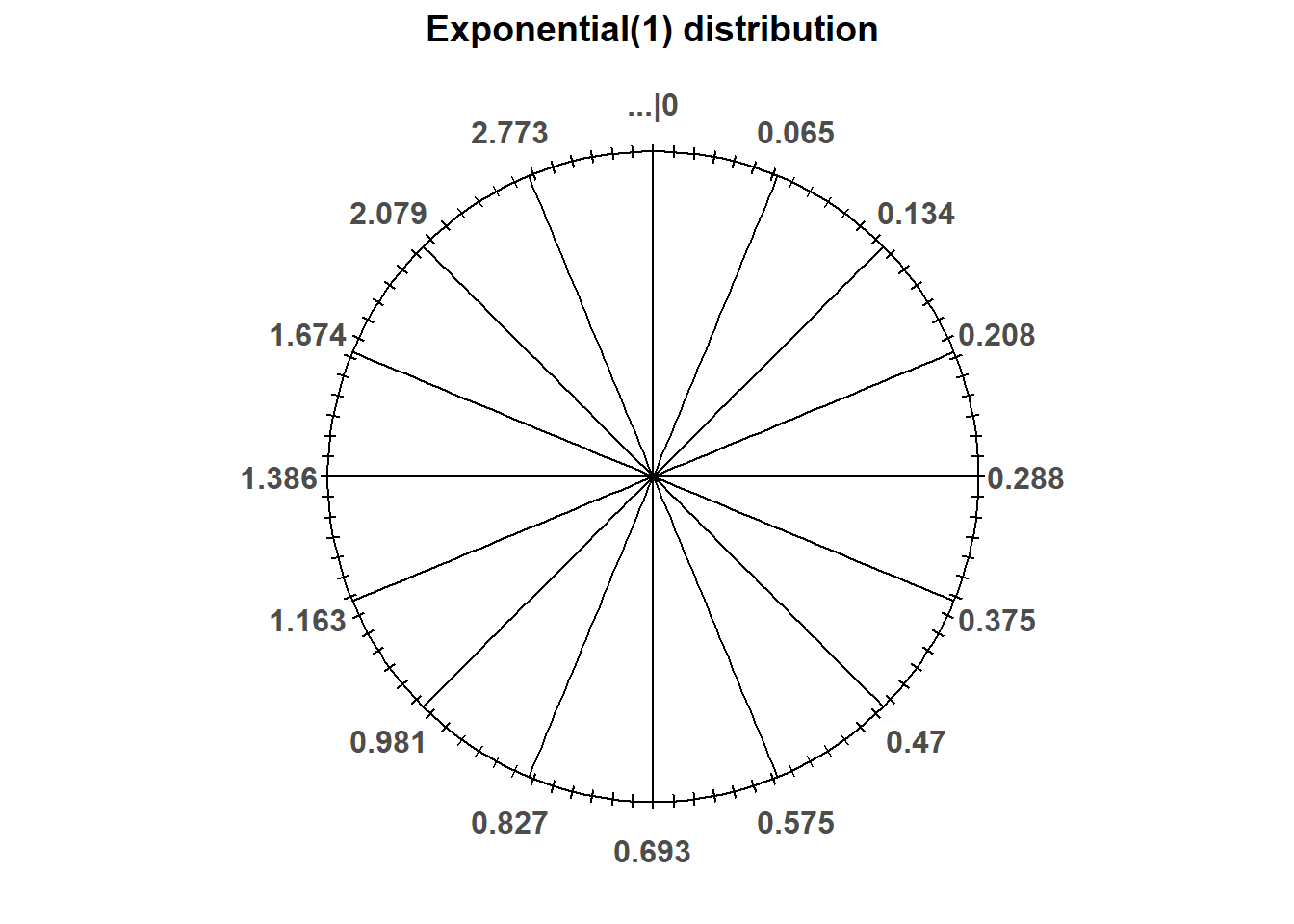
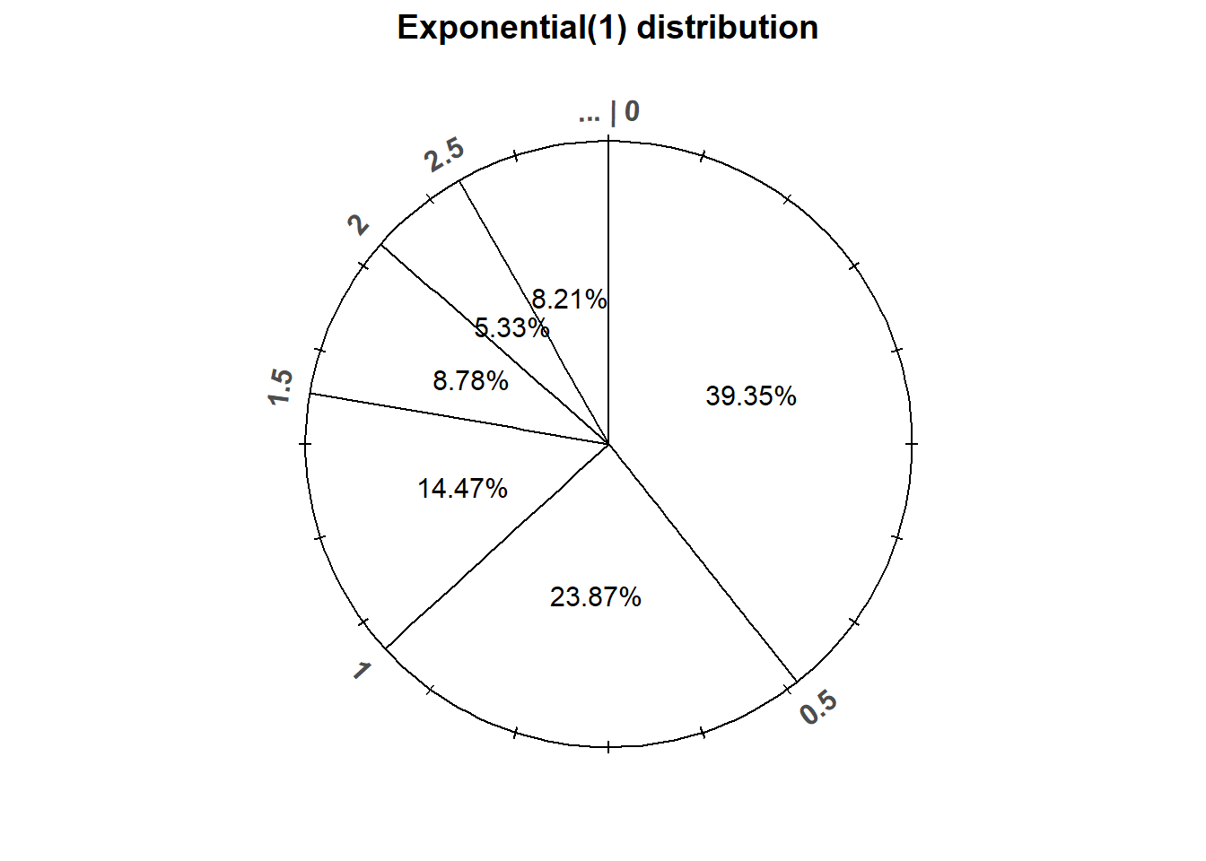
Figure 4.13: An Exponential(1) spinner. The same spinner is displayed on both sides, with different features highlighted on the left and right. Only selected rounded values are displayed, but in the idealized model the spinner is infinitely precise so that any real number greater than 0 is possible. Notice that the values on the axis are not evenly spaced.

4.3.1 Uniform distributions

In general, a pdf \(f_X(x)\) depends on the value \(x\) of the random variable \(X\). Uniform distributions are a special case where the pdf is constant for all possible values.

Example 4.10 In the meeting problem assume that Regina’s arrival time \(X\) (minutes after noon) follows a Uniform(0, 60) distribution.

1. Sketch a plot of the pdf of \(X\).
2. Donny Dont says that the pdf is \(f_X(x) = 1/60\). Do you agree? If not, specify the pdf of \(X\).
3. Use the pdf to find the probability that Regina arrives before 12:15.
4. Use the pdf to find the probability that Regina arrives after 12:45.
5. Use the pdf to find the probability that Regina arrives between 12:15 and 12:45.
6. Use the pdf to find the probability that Regina arrives between 12:15:00 and 12:16:00.
7. Use the pdf to find the probability that Regina arrives between 12:15:00 and 12:15:01.
8. Use the pdf to find the probability that Regina arrives at the exact time 12:15:00 (with infinite precision).

Solution. to Example 4.10

Show/hide solution

Note: in a situation like this, you should use properties of Uniform distributions, sketch pictures, and use geometry to solve problems. That is, you should not immediately resort to calculus. However, we show the calculus below to illustrate ideas, and because we have tackled this problem previously with Uniform probability measures and geometry in Example 3.29.

1. We expect the height of the pdf to be constant between 0 and 60, both because her arrival time is uniform over the interval so no one value should be more likely than another, and because when we simulated values the histogram bars had roughly constant height. See the plot below.
2. We need the area under the curve over the interval \([0, 60]\) to be 1, representing 100% probability. If the height of the density is \(c\), a constant, then the area under the curve is the area of a rectangle with base 60 (length of the interval \([0, 60]\)) and height \(c\). So \(c\) needs to be 1/60 for the total area to be 1.
   However, Donny Don’t hasn’t specified the possible values. It’s possible that someone who sees Donny’s expression would think that \(f_X(100)=1/60\). But the pdf is only 1/60 over the range \([0, 60]\); it is 0 outside of this range. A more precise expression is \[ f_X(x) = \begin{cases} 1/60, & 0\le x \le 60,\\ 0, & \text{otherwise.} \end{cases} \] You don’t necessarily always need to write “0 otherwise”, but do always provide the possible values.
3. Integrate the pdf over the range \([0, 15]\). Since the pdf has constant height, areas under the curve just correspond to areas of rectangles. \[ \textrm{P}(X \le 15) = \int_0^{15} (1/60) dx = (1/60)x\Big|_{x = 0}^{x = 15} = \frac{15}{60} = 0.25 \]
4. Integrate the pdf over the range \([45, 60]\).
   \[ \textrm{P}(X \ge 45) = \int_{45}^{60} (1/60) dx = (1/60)x\Big|_{x = 45}^{x = 60} = \frac{15}{60} = 1-0.75 = 0.25 \]
5. We could use the previous parts, but we’ll intergrate the pdf over the range \([15, 45]\). \[ \textrm{P}(15 \le X \le 45) = \int_{15}^{45} (1/60) dx = (1/60)x\Big|_{x = 15}^{x = 45} = \frac{30}{60} = 0.75 -0.25 = 0.5 \].
6. Integrate the pdf over the range \([15, 15 + 1]\).
   \[ \textrm{P}(15 \le X \le 15 + 1) = (1/60)(1) = 1/60 \]
7. Integrate the pdf over the range \([15, 15 + 1/60]\).
   \[ \textrm{P}(15 \le X \le 15 + 1/60) = (1/60)(1/60) = 1/3600 \]
8. \(\textrm{P}(X = 15) = 0\). Integrate the pdf over the range \([15, 15]\). The region under the curve at this single point corresponds to a line segment which has 0 area. \[ \textrm{P}(X = 15) = \int_{15}^{15} (1/60) dx = 0 \]

Figure 4.14: The pdf of a Uniform(0, 60) distribution. The blue line represents the pdf. The shaded orange region represents the probability of the interval [15, 45].

Example 4.11 Suppose that SAT Math scores follow a Uniform(200, 800) distribution. Let \(U\) be the Math score for a randomly selected student.

1. Identify \(f_U\), the pdf of \(U\).
2. Donny Dont says that the probability that \(U\) is 500 is 1/600. Do you agree? If not, explain why not.
3. While modeling SAT Math score as a continuous random variable might be mathematically convenient, it’s not entirely practical. Suppose that the range of values \([495, 505)\) corresponds to students who actually score 500. Find \(\textrm{P}(495 \le X < 505)\).

Solution. to Example 4.11

Show/hide solution

1. The density still has constant height. But now the height has to be 1/600 so that the total area under the pdf over the range of possible values \([200, 800]\) is 1. So \(f_U(u) = \frac{1}{600}, 200<u<800\) (and \(f_U(u)=0\) otherwise).
2. It is true that \(f_U(500)=1/600\). However, \(f_U(500)\) is NOT \(\textrm{P}(U=500)\). The density (height) at a particular point is not the probability of anything. Probabilities are determined by integrating the density. The “area” under the curve for the region \([500,500]\) is just a line segment, which has area 0, so \(\textrm{P}(U=500)=0\). Integrating, \(\int_{500}^{500}(1/600)du=0\). More on this point below.
3. \(\textrm{P}(495 \le U < 505)=(505-495)(1/600) = 1/60\). The integral \(\int_{495}^{505}(1/600)du\) corresponds to the area of a rectangle with base \(505-495\) and height 1/600, so the area is 1/60.

Definition 4.5 A continuous random variable \(X\) has a Uniform distribution with parameters \(a\) and \(b\), with \(a<b\), if its probability density function \(f_X\) satisfies \[\begin{align*} f_X(x) & \propto \text{constant}, \quad & & a<x<b\\ & = \frac{1}{b-a}, \quad & & a<x<b. \end{align*}\] If \(X\) has a Uniform(\(a\), \(b\)) distribution then \[\begin{align*} \text{Long run average value of $X$} & = \frac{a+b}{2}\\ \text{Variance of $X$} & = \frac{|b-a|^2}{12}\\ \text{SD of $X$} & = \frac{|b-a|}{\sqrt{12}} \end{align*}\]

The long run average value of a random variable that has a Uniform(\(a\), \(b\)) distribution is the midpoint of the range of possible values. The degree of variability of a Uniform distribution is determined by the length of the interval. Why is the standard deviation equal to the length of the interval multiplied by \(0.289 \approx 1/\sqrt{12}\)? Since the deviations from the mean (midpoint) range uniformly from 0 to half the length of the interval, we might expect the average deviation to be about 0.25 times the length of the interval. The factor \(0.289 \approx 1/\sqrt{12}\), which results from the process of taking the square root of the average of the squared deviations, is not too far from 0.25.

The “standard” Uniform distribution is the Uniform(0, 1) distribution represented by the spinner in Figure 2.1. If \(U\) has a Uniform(0, 1) distribution then \(X = a + (b-a)U\) has a Uniform(\(a\), \(b\)) distribution. Notice that the linear rescaling of \(U\) to \(a + (b-a)U\) does not change the basic shape of the distribution, just the region of possible values. Therefore, we can construct a spinner for any Uniform distribution by starting with the Uniform(0, 1) and linearly rescaling the values on the spinner axis.

4.3.2 Density is not probability

Plugging a value into the pdf of a continuous random variable does not provide a probability. The pdf itself does not provide probabilities directly; instead a pdf must be integrated to find probabilities.

The probability that a continuous random variable \(X\) equals any particular value is 0. That is, if \(X\) is continuous then \(\textrm{P}(X=x)=0\) for all \(x\). Therefore, for a continuous random variable¹⁰⁵, \(\textrm{P}(X\le x) = \textrm{P}(X<x)\), etc. A continuous random variable can take uncountably many distinct values. Simulating values of a continuous random variable corresponds to an idealized spinner with an infinitely precise needle which can land on any value in a continuous scale.

In the Uniform(0, 1) case, \(0.500000000\ldots\) is different than \(0.50000000010\ldots\) is different than \(0.500000000000001\ldots\), etc. Consider the spinner in Figure 2.1. The spinner in the picture is only labeled in 100 increments of 0.01 each; when we spin, the probability that the needle lands closest to the 0.5 tick mark is 0.01. But if the spinner were labeled in increments 1000 increments of 0.001, the probability of landing closest to the 0.5 tick mark is 0.001. And with four decimal places of precision, the probability is 0.0001. And so on. The more precise we mark the axis, the smaller the probability the spinner lands closest to the 0.5 tick mark. The Uniform(0, 1) density represents what happens in the limit as the spinner becomes infinitely precise. The probability of landing closest to the 0.5 tick mark gets smaller and smaller, eventually becoming 0 in the limit.

A density is an idealized mathematical model. In practical applications, there is some acceptable degree of precision, and events like “\(X\), rounded to 4 decimal places, equals 0.5” correspond to intervals that do have positive probability. For continuous random variables, it doesn’t really make sense to talk about the probability that the random value is equal to a particular value. However, we can consider the probability that a random variable is close to a particular value.

Example 4.12 Continuing Example 4.10, we will now we assume Regina’s arrival time in \([0, 1]\) has pdf

\[ f_X(x) = \begin{cases} cx, & 0\le x \le 1,\\ 0, & \text{otherwise.} \end{cases} \]

where \(c\) is an appropriate constant.

Note that now we’re measuring arrival time in hours (i.e., fraction of the hour after noon) instead of minutes.

1. Sketch a plot of the pdf. What does this say about Regina’s arival time?
2. Find the value of \(c\) and specify the pdf of \(X\).
3. Find the probability that Regina arrives before 12:15.
4. Find the probability that Regina arrives after 12:45. How does this compare to the previous part? What does that say about Regina’s arrival time?
5. Find the probability that Regina arrives between 12:15 and 12:45.
6. Find the probability that Regina arrives between 12:15 and 12:16.
7. Find the probability that Regina arrives between 12:15:00 and 12:15:01.
8. Find the probability that Regina arrives at the exact time 12:15:00 (with infinite precision).
9. Find the probability that Regina arrives between 12:59:00 and 1:00:00. How does this compare to the probability for 12:15:00 to 12:16:00? What does that say about Regina’s arrival time?
10. Find the probability that Regina arrives between 12:59:59 and 1:00:00. How does this compare to the probability for 12:15:00 to 12:15:01? What does that say about Regina’s arrival time?
11. Find the probability that Regina arrives at the exact time 1:00:00 (with infinite precision).
12. Compare this example and your answers to Example 3.31.

Solution. to Example 4.12

Show/hide solution

You should always start problems like this by drawing the pdf and shading regions corresponding to probabilities. In some cases, areas can be determine by simple geometry without needing calculus. We have included the integrals below for completeness, but make sure you also see how the probabilities can be determined using geometry.

1. The density increases linearly with \(x\). Regina is most likely to arrive closer to 1, and least likely to arrive close to noon (0).
2. \(c=2\). The total area under the pdf must be 1. The region under the pdf is a triangle with area \((1/2)(1-0)(c)\), so \(c\) must be 2 for the area to be 1. Via integration \[ 1 = \int_0^1 cx dx = (c/2)x^2 \Big|_{x=0}^{x=1} = c / 2 \]
3. Integrate the pdf over the region \([0, 0.25]\). Since the pdf is linear, regions under the curve are triangles or trapezoids. The area corresponding to [0, 0.25] is a triangle with base (0.25 - 0), height \(c(0.25) = 2(0.25)\), and area \(0.5(0.25-0)(2(0.25)) = 0.25^2 = 0.0625\). \[ \int_0^{0.25} 2x dx = x^2 \Bigg|_{x=0}^{x=0.25} = 0.25^2 = (1/2)(0.25 - 0)(2(0.25)) = 0.0625 \]
4. Integrate the pdf over the region \([0.75, 1]\). \[ \int_{0.75}^1 2x dx = x^2 \Bigg|_{x=0.75}^{x=1} = 1 - 0.75^2 = 0.4375 \] So Regina is 7 times more likely to arrive within 15 minutes of 1 than within 15 minutes of noon.
5. 0.5. We could integrate the pdf from 0.25 to 0.75, or just use the previous results and properties of probabilities.
6. Similar to the previous parts, the probability is \((0.25 + 1/60)^2 - 0.25^2 = 0.0086\). (This probability is less than what it was in the uniform case.)
7. Similar to the previous part, \((0.25 + 1/3600)^2 - 0.25^2 = 0.00014\). (This probability is less than what it was in the uniform case.)
8. The exact time 12:15:00 represents a single point the sample space, an interval of length 0. The probability that Regina arrives at the exact time 12:15:00 (with infinite precision) is 0.
9. Similar to previous parts, \(1^2 - (1-1/60)^2 = 0.0331\). Notice that this one minute interval around 1:00 has a probability that is about 3.85 times larger than a one minute interval around 12:15.
10. \(1^2 - (1-1/3600)^2 = 0.00056\). Notice that this one second interval around 1:00 has a probability that is about 4 times higher than a one second interval around 12:15, though both probabilities are small.
11. The exact time 1:00:00 represents a single point the sample space, an interval of length 0. The probability that Regina arrives at the exact time 1:00:00 (with infinite precision) is 0.
12. The results are the same as those in Example 3.31. In that example, the probability that Regina arrives in the interval \([0, x]\) was \(x^2\), which can be obtained by integrating the pdf in this example from 0 to \(x\). Careful when you integrate; since \(x\) is in the bounds of the integral you need a different dummy variable to use in \(f_X\). \[ \textrm{P}(X \le x) = \int_0^x f_X(u) du = \int_0^x 2u du = u^2 \Bigg|_{u=x}^{u=0} = x^2 \] We will see soon that such a function is called a cumulative distribution function (cdf).

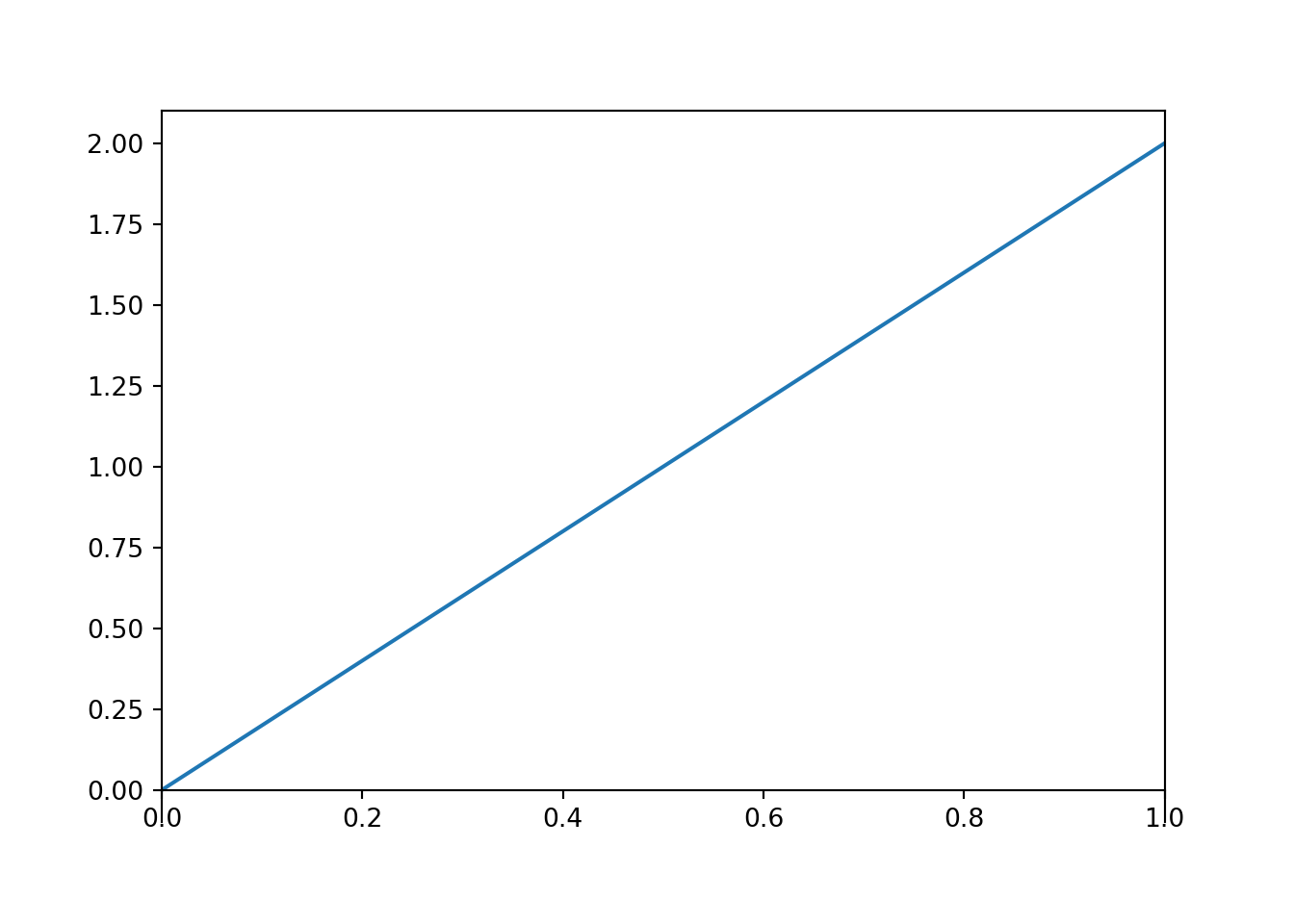
Figure 4.15: The probability density function from Example 4.12.

In the previous example, we specified the general shape of the pdf, then found the constant that made the total area under the curve equal to 1. In general, a pdf is often defined only up to some multiplicative constant \(c\), for example \(f_X(x) = c\times(\text{some function of }x)\), or \(f_X(x) \propto \text{some function of }x\). The constant \(c\) does not affect the shape of the distribution as a function of \(x\), only the scale on the density axis. The absolute scaling on the density axis is somewhat irrelevant; it is whatever it needs to be to provide the proper area. In particular, the total area under the pdf must be 1. The scaling constant is determined by the requirement that \(\int_{-\infty}^\infty f_X(x) dx = 1\).

What’s more important about the pdf is relative heights. In the previous example the density at 1, \(f_X(1) = c\), was 4 times greater than than density at 0.25, \(f_X(0.25) = 0.25c\). This was the reason why the probability of arriving close to 1 was about 4 times greater than the probability of arriving close to 12:15 (time 0.25). The ratio of the densities at these two points could be computed without knowing the value of \(c\).

Compare the pdf in Example 4.15 with the probabilities under the non-uniform measure in Figure 3.7. The pdf at a particular possible value \(x\) is related to the probability that the random value takes a value close to that value \(x\).

Example 4.13 Let \(X\) be a random variable with the “Exponential(1)” distribution, illustrated by the smooth curve in Figure 4.11. Then the pdf of \(f_X\) is

\[ f_X(x) = \begin{cases} e^{-x}, & x>0,\\ 0, & \text{otherwise.} \end{cases} \]

1. Compute \(\textrm{P}(X = 1)\).
2. Without integrating, approximate the probability that \(X\) rounded to two decimal places is 1.
3. Without integrating, approximate the probability that \(X\) rounded to two decimal places is 1.7.
4. Find and interpret the ratio of the probabilities from the two previous parts. How could we have obtained this ratio from the pdf?

Solution. to Example 4.13

Show/hide solution

1. \(\textrm{P}(X = 1)=0\), since \(X\) is continuous.
2. Over a short region around 1, the area under the curve can be approximated by the area of a rectangle with height \(f_X(1)\): \[ \textrm{P}(0.995<X<1.005)\approx f_X(1)(1.005 - 0.995)=e^{-1}(0.01)\approx 0.00367879. \] See the illustration below. This provides a pretty good approximation of the true integral¹⁰⁶ \(\int_{0.995}^{1.005} e^{-x}dx = e^{-0.995}-e^{-1.005}\approx 0.00367881\).
3. Over a short region around 1.7, the area under the curve can be approximated by the area of a rectangle with height \(f_X(1.7)\): \[ \textrm{P}(1.695<X<1.705)\approx f_X(1.7)(1.705 - 1.695)=e^{-1.7}(0.01)\approx 0.001826835. \] This provides a pretty good approximation of the integral \(\int_{1.695}^{1.705} e^{-x}dx = e^{-1.695}-e^{-1.705}\approx 0.001826843\).
4. Compare the rectangle-based approximations \[ \frac{\textrm{P}(1 - 0.005 <X < 1 + 0.005)}{\textrm{P}(1.7 - 0.005 <X < 1.7 + 0.005)} \approx 2.01 \approx \frac{e^{-1}(0.01)}{e^{-1.7}(0.01)} = \frac{e^{-1}}{e^{-1.7}} = \frac{f_X(1)}{f_X(1.7)} \] The probability that \(X\) is “close to” 1 is about 2 times greater than the probability that \(X\) is “close to” 1.7. This ratio is determined by the ratio of the densities at 1 and 1.7.

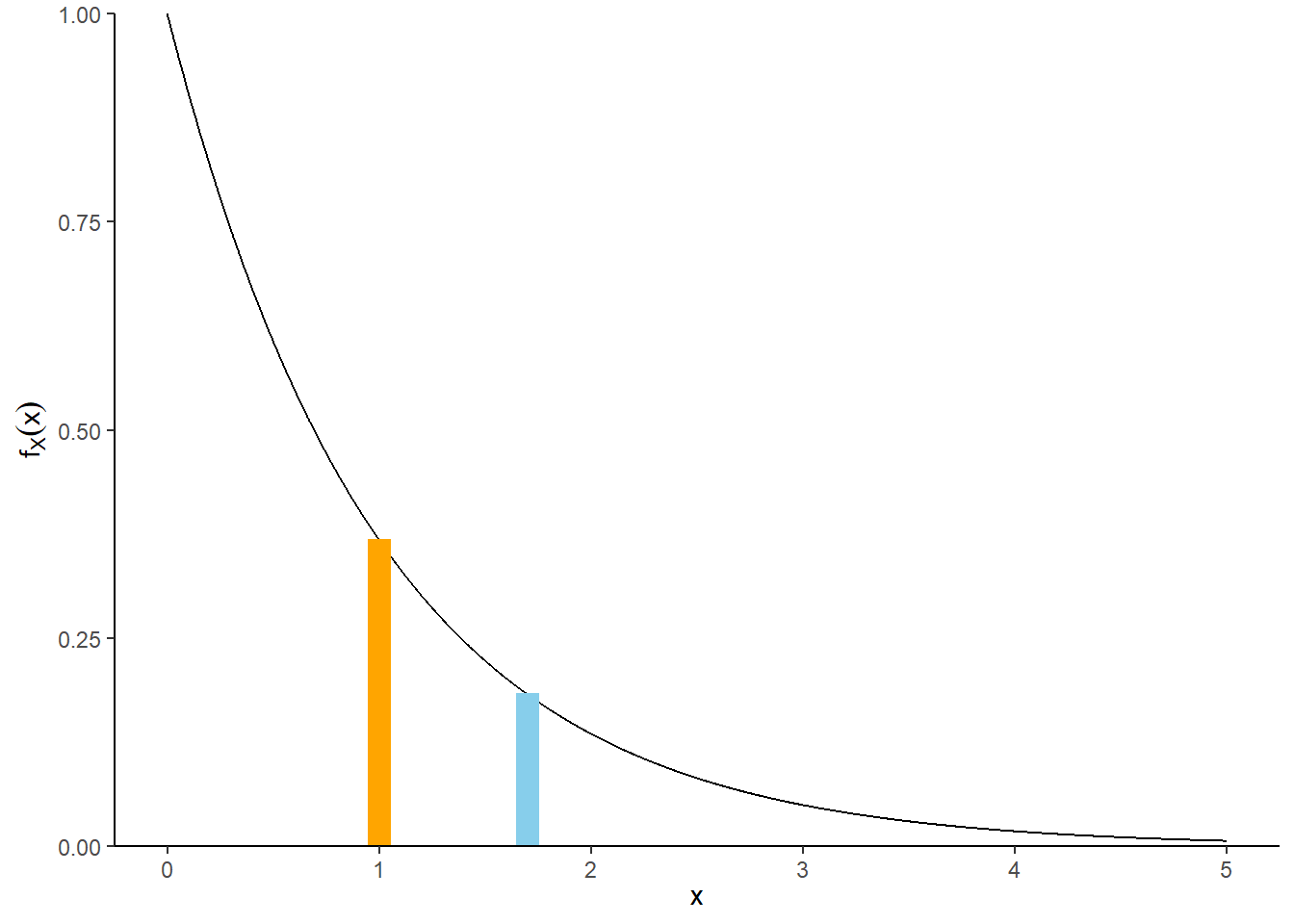
Figure 4.16: Illustration of \(\textrm{P}(0.995<X<1.005)\) (orange) and \(\textrm{P}(1.695<X<1.705)\) (blue) for \(X\) with an Exponential(1) distribution. The plot illustrates how the probability that \(X\) is “close to” \(x\) can be approximated by the area of a rectangle with height equal to the density at \(x\), \(f_X(x)\). The density height at \(x = 1\) is roughly twice as large than the density height at \(x = 1.7\) so the probability that \(X\) is “close to” 1 is (roughly) twice as large as the probability that \(X\) is “close to” 1.7.

A density is an idealized mathematical model. In practical applications, there is some acceptable degree of precision, and events like “\(X\), rounded to 4 decimal places, equals 0.5” correspond to intervals that do have positive probability. For continuous random variables, it doesn’t really make sense to talk about the probability that the random value equals a particular value. However, we can consider the probability that a random variable is close to a particular value.

To emphasize: The density \(f_X(x)\) at value \(x\) is not a probability. Rather, the density \(f_X(x)\) at value \(x\) is related to the probability that the RV \(X\) takes a value “close to \(x\)” in the following sense¹⁰⁷. \[ \textrm{P}\left(x-\frac{\epsilon}{2} \le X \le x+\frac{\epsilon}{2}\right) \approx f_X(x)\epsilon, \qquad \text{for small $\epsilon$} \] The quantity \(\epsilon\) is a small number that represents the desired degree of precision. For example, rounding to two decimal places corresponds to \(\epsilon=0.01\).

Technically, any particular \(x\) occurs with probability 0, so it doesn’t really make sense to say that some values are more likely than others. However, a RV \(X\) is more likely to take values close to those values that have greater density. As we said previously, what’s important about a pdf is relative heights. For example, if \(f_X(x_2)= 2f_X(x_1)\) then \(X\) is roughly “twice as likely to be near \(x_2\) than to be near \(x_1\)” in the above sense. \[ \frac{f_X(x_2)}{f_X(x_1)} = \frac{f_X(x_2)\epsilon}{f_X(x_1)\epsilon} \approx \frac{\textrm{P}\left(x_2-\frac{\epsilon}{2} \le X \le x_2+\frac{\epsilon}{2}\right)}{\textrm{P}\left(x_1-\frac{\epsilon}{2} \le X \le x_1+\frac{\epsilon}{2}\right)} \]

4.3.3 Exponential distributions

Exponential distributions are often used to model the waiting times between events in a random process that occurs continuously over time.

Example 4.14 Suppose that we model the waiting time, measured continuously in hours, from now until the next earthquake (of any magnitude) occurs in southern CA as a continuous random variable \(X\) with pdf \[ f_X(x) = 2 e^{-2x}, \; x \ge0 \] This is the pdf of the “Exponential(2)” distribution.

1. Sketch the pdf of \(X\). What does this tell you about waiting times?
2. Without doing any integration, approximate the probability that \(X\) rounded to the nearest minute is 0.5 hours.
3. Without doing any integration determine how much more likely that \(X\) rounded to the nearest minute is to be 0.5 than 1.5.
4. Compute and interpret \(\textrm{P}(X > 0.25)\).
5. Compute and interpret \(\textrm{P}(X \le 3)\).
6. Compute and interpret the 25th percentile of \(X\).
7. Compute and interpret the 50th percentile of \(X\).
8. Compute and interpret the 75th percentile of \(X\).
9. How do the values from the three previous parts compare to the percentiles from the Exponential(1) distribution depicted in 4.13? Suggest a method for simulating values of \(X\) using the Exponential(1) spinner.
10. Use simulation to approximate the long run average value of \(X\). Interpret this value. At what rate do earthquakes tend to occur?
11. Use simulation to approximate the standard deviation of \(X\). What do you notice?

Solution. to Example 4.14

Show/hide solution

1. See simulation below for plots. Waiting times near 0 are most likely, and density decreases exponentially as waiting time increases.
2. Remember, the density at \(x=0.5\) is not a probability, but it is related to the probability that \(X\) takes a value close to \(x=0.5\). The approximate probability that \(X\) rounded to the nearest minute is 0.5 hours is \[ f_X(0.5)(1/60) = 2e^{-2(0.5)}(1/60) = 0.0123 \]
3. Find the ratio of the densities at 0.5 and 1.5: \[ \frac{f_X(0.5)}{f_X(1.5)} = \frac{2e^{-2(0.5)}}{2e^{-2(1.5)}} = \frac{e^{-2(0.5)}}{e^{-2(1.5)}} \approx 7.4. \] \(X\) rounded to the nearest minute is about 7.4 times more likely to be 0.5 than 1.5. A waiting time close to half an hour is about 7.4 times more likely than a waiting time close to 1.5 hours.
4. \(\textrm{P}(X > 0.25) = \int_{0.25}^\infty 2e^{-2x}dx = e^{-2(0.25)}=0.606\). Careful: this is not \(2e^{-2(0.25)}\). According to this model, the waiting time between earthquakes is more than 15 minutes for about 60% of earthquakes.
5. \(\textrm{P}(X \le 3) = \int_0^3 2e^{-2x}dx = 1-e^{-2(3)}=0.9975\). While any value greater than 0 is possible in principle, the probability that \(X\) takes a really large value is small. About 99.75% of earthquakes happen within 3 hours of the previous earthquake.
6. We want to find \(x>0\) such that \(\textrm{P}(X \le x) =0.25\): \[ 0.25 = \textrm{P}(X \le x) = \int_0^{x} 2e^{-2u}du = 1 - e^{-2x} \] Solve to get \(x = -0.5\log(1-0.25) = 0.5(0.288)=0.144\). For 25% of earthquakes, the next earthquake happens within 0.144 hours (8.6 minutes). Constructing a spinner, the value \(0.5(0.288)=0.144\) goes at 3 o’clock on the spinner axis.
7. We want to find \(x>0\) such that \(\textrm{P}(X \le x) =0.5\): \[ 0.5 = \textrm{P}(X \le x) = \int_0^{x} 2e^{-2u}du = 1 - e^{-2x} \] Solve to get \(x = -0.5\log(1-0.5) = 0.5(0.693)=0.347\). For 50% of earthquakes, the next earthquake happens within 0.347 hours (20.8 minutes). Constructing a spinner, the value \(0.5(0.693)=0.347\) goes at 6 o’clock on the spinner axis.
8. We want to find \(x>0\) such that \(\textrm{P}(X \le x) =0.75\): \[ 0.75 = \textrm{P}(X \le x) = \int_0^{x} 2e^{-2u}du = 1 - e^{-2x} \] Solve to get \(x = -0.5\log(1-0.75) = 0.5(1.386)=0.693\). For 75% of earthquakes, the next earthquake happens within 0.693 hours (41.6 minutes). Constructing a spinner, the value \(0.5(1.386)=0.693\) goes at 9 o’clock on the spinner axis.
9. We could construct a spinner corresponding to an Exponential(2) distribution. But the previous parts suggest that the values on the axis of the Exponential(2) are the values on the Exponential(1) spinner multiplied by 1/2. For example, for an Exponential(1) distribution 25% of values are less than 0.288, while for an Exponential(2) distribution 25% of values are less than \(0.5(0.288) = 0.144\). Therefore, to simulate a value from an Exponential(2) distribution we can simulate a value from an Exponential(1) distribution and multiply the result by 1/2.
10. See simulation results below. The simulated average is about 0.5 hours. According to this model, the average waiting time between earthquakes is 0.5 hours. That is, earthquakes tend to occur at rate 2 earthquakes per hour on average; this is what the parameter 2 in the pdf represents.
11. The simulated standard deviation is also about 0.5, the same as the long run average value.

Below we simulate values from an Exponential distribution with rate parameter 2 and compare the simulated values to the theoretical results. In Symbulate .cdf() returns \(\le\) probabilities; for example Exponential(2).cdf(3) returns the probability that a random variable with an Exponential(2) distribution takes a value \(\le 3\). (We will discuss cdfs in more detail in the next section.)

X = RV(Exponential(rate = 2))

x = X.sim(10000)

x

Index	Result
0	1.1441042094179017
1	0.6782965508631741
2	0.1905848350905949
3	0.5365659147759795
4	0.5774724245898746
5	0.039921529764954986
6	0.5816425565273713
7	0.3357083155311557
8	0.7393400397711187
...	...
9999	0.1811547623320253

x.plot() # plot the simulated values

Exponential(rate = 2).plot() # plot the theoretical Exponential(2) pdf

x.count_gt(0.25) / x.count(), 1 - Exponential(rate = 2).cdf(0.25)

## (0.5963, 0.6065306597126334)

x.count_lt(3) / x.count(), Exponential(rate = 2).cdf(3)

## (0.9971, 0.9975212478233336)

x.mean(), Exponential(rate = 2).mean()

## (0.4929953342656256, 0.5)

x.sd(), Exponential(rate = 2).sd()

## (0.503552132185389, 0.5)

Definition 4.6 A continuous random variable \(X\) has an Exponential distribution with rate parameter¹⁰⁸ \(\lambda>0\) if its pdf is \[ f_X(x) = \begin{cases}\lambda e^{-\lambda x}, & x \ge 0,\\ 0, & \text{otherwise} \end{cases} \] If \(X\) has an Exponential(\(\lambda\)) distribution then \[\begin{align*} \textrm{P}(X>x) & = e^{-\lambda x}, \quad x\ge 0\\ \text{Long run average of $X$} & = \frac{1}{\lambda}\\ \text{Standard deviation of $X$} & = \frac{1}{\lambda} \end{align*}\]

Exponential distributions are often used to model the waiting time in a random process until some event occurs.

• \(\lambda\) is the average rate at which events occur over time (e.g., 2 per hour)
• \(1/\lambda\) is the mean time between events (e.g., 1/2 hour)

An Exponential density has a peak at 0 and then decreases exponentially as \(x\) increases. The function \(e^{-\lambda x}\) defines the shape of the density and the rate at which the density decreases. The constant \(\lambda\), which defines the density at \(x=0\), simply rescales the vertical axis so that the total area under the pdf is 1.

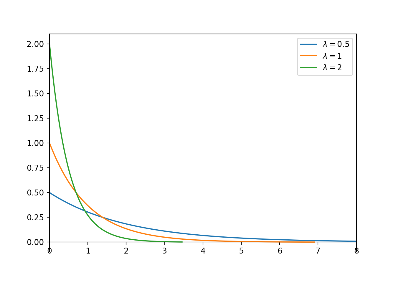
Figure 4.17: Exponential densities with rate parameter \(\lambda\).

The “standard” Exponential distribution is the Exponential(1) distribution, with rate parameter 1 and long run average 1. If \(X\) has an Exponential(1) distribution and \(\lambda>0\) is a constant then \(X/\lambda\) has an Exponential(\(\lambda\)) distribution. Recall that an Exponential(\(\lambda\)) distribution has long run average value \(1/\lambda\). Values from an Exponential(1) distribution will have long run average value 1, so if we multiply all the values by \(1/\lambda\) then the transformed values will have long run average value \(1/\lambda\). Multiplying by the constant \(1/\lambda\) does not change the shape of the distribution; it just relabels the values on the variable axis.

U = RV(Exponential(1))

X = (1 / 2) * U

X.sim(10000).plot()  # simulated distribution of X

Exponential(rate = 2).plot() # theoretical distribution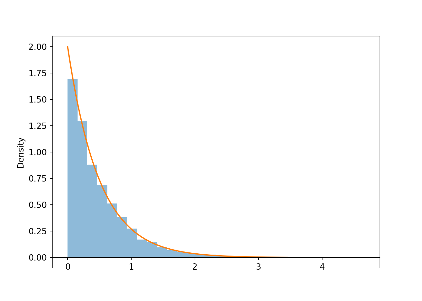

---

105. The same is not true for discrete random variables. For example, if \(X\) is the number of heads in three flips of a fair coin then \(\textrm{P}(X<1)= \textrm{P}(X=0)=1/8\) but \(\textrm{P}(X \le 1)=\textrm{P}(X=0)+\textrm{P}(X=1) = 4/8\).↩︎

106. Reporting so many decimal places is unnecessary, and provides a false sense of precision. All of these idealized mathematical models are at best approximately true in practice. However, we provide the extra decimal places here to compare the approximation with the “exact” calculation.↩︎

107. This is true because an integral can be approximated by a sum of the areas of many rectangles with narrow bases. Over a small interval of values surrounding \(x\), the density shouldn’t change that much, so we can estimate the area under the curve by the area of the rectangle with height \(f_X(x)\) and base each equal to the length of the small interval of interest.↩︎

108. Exponential distributions are sometimes parametrized directly by their mean \(1/\lambda\), instead of the rate parameter \(\lambda\). The mean \(1/\lambda\) is sometimes called the scale parameter.↩︎