5.5 Expected values of linear combinations of random variables
Remember that, in general, you cannot interchanging averaging and transformation. In general, an expected value of a function of random variables is not the function evaluated at the expected values of the random variables.
\[\begin{align*} \textrm{E}(g(X)) & \neq g(\textrm{E}(X)) & & \text{for most functions $g$}\\ \textrm{E}(g(X, Y)) & \neq g(\textrm{E}(X), \textrm{E}(Y)) & & \text{for most functions $g$} \end{align*}\]
But there are some functions, namely linear functions, for which an expected value of the transformation is the transformation evaluated at the expected values. In this section, we will study “linearity of expected value” and applications. We will also investigate variance of linear transformations of random variables, and in particular, the role that covariance plays.
5.5.1 Linear rescaling
A linear rescaling is a transformation of the form \(g(u) = au + b\). Recall that in Section 4.6.1 we observed, via simulation, that
- A linear rescaling of a random variable does not change the basic shape of its distribution, just the range of possible values.
- A linear rescaling transforms the mean in the same way the individual values are transformed.
- Adding a constant to a random variable does not affect its standard deviation.
- Multiplying a random variable by a constant multiples its standard deviation by the absolute value of the constant.
If \(X\) is a random variable and \(a, b\) are non-random constants then
\[\begin{align*} \textrm{E}(aX + b) & = a\textrm{E}(X) + b\\ \textrm{SD}(aX + b) & = |a|\textrm{SD}(X)\\ \textrm{Var}(aX + b) & = a^2\textrm{Var}(X) \end{align*}\]
5.5.2 Linearity of expected value
Example 5.28 Spin the Uniform(1, 4) spinner twice and let \(U_1\) be the first spin, \(U_2\) the second, and \(X = U_1 + U_2\) the sum.
- Find \(\textrm{E}(U_1)\) and \(\textrm{E}(U_2)\).
- Find \(\textrm{E}(X)\).
- How does \(\textrm{E}(X)\) relate to \(\textrm{E}(U_1)\) and \(\textrm{E}(U_2)\)? Suggest a simpler way of finding \(\textrm{E}(U_1 + U_2)\).
Show/hide solution
- \(\textrm{E}(U_1) = \frac{1+4}{2} = 2.5 = \textrm{E}(U_2)\).
- We found the pdf of \(X\) in Example 4.36. Since the pdf of \(X\) is symmetric about \(5\) we should have \(\textrm{E}(X)=5\), which integrating confirms. \[ \textrm{E}(X) = \int_2^5 x \left((x-2)/9\right)dx + \int_5^8 x \left((8-x)/9\right) dx = 5. \]
- We see that \(\textrm{E}(U_1+U_2) = 5 = 2.5 + 2.5 = \textrm{E}(U_1) + \textrm{E}(U_2)\). Finding the expected value of each of \(U_1\) and \(U_2\) and adding these two numbers is much easier than finding the pdf of \(U_1+U_2\) and then using the definition of expected value.
In the previous example, the values \(U_1\) and \(U_2\) came from separate spins so they were uncorrelated (in fact, they were independent). What about the expected value of \(X+Y\) when \(X\) and \(Y\) are correlated?
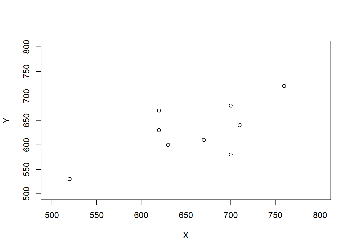
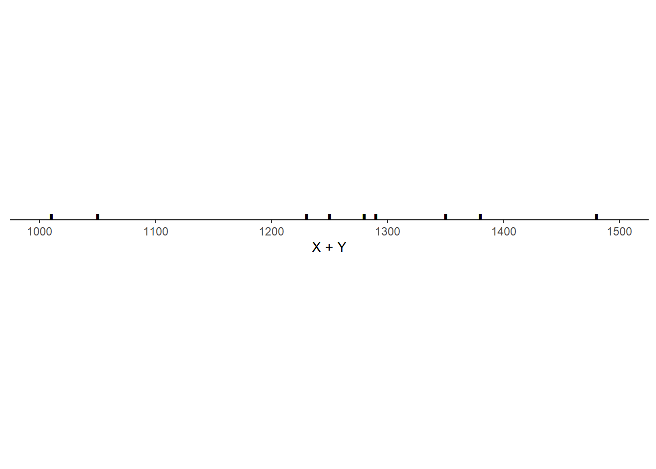
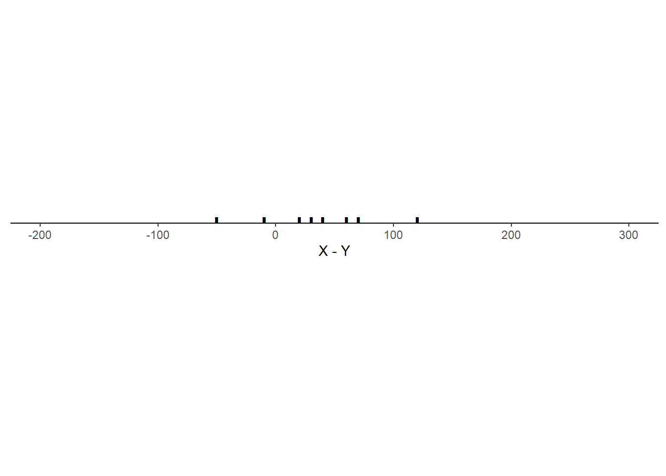
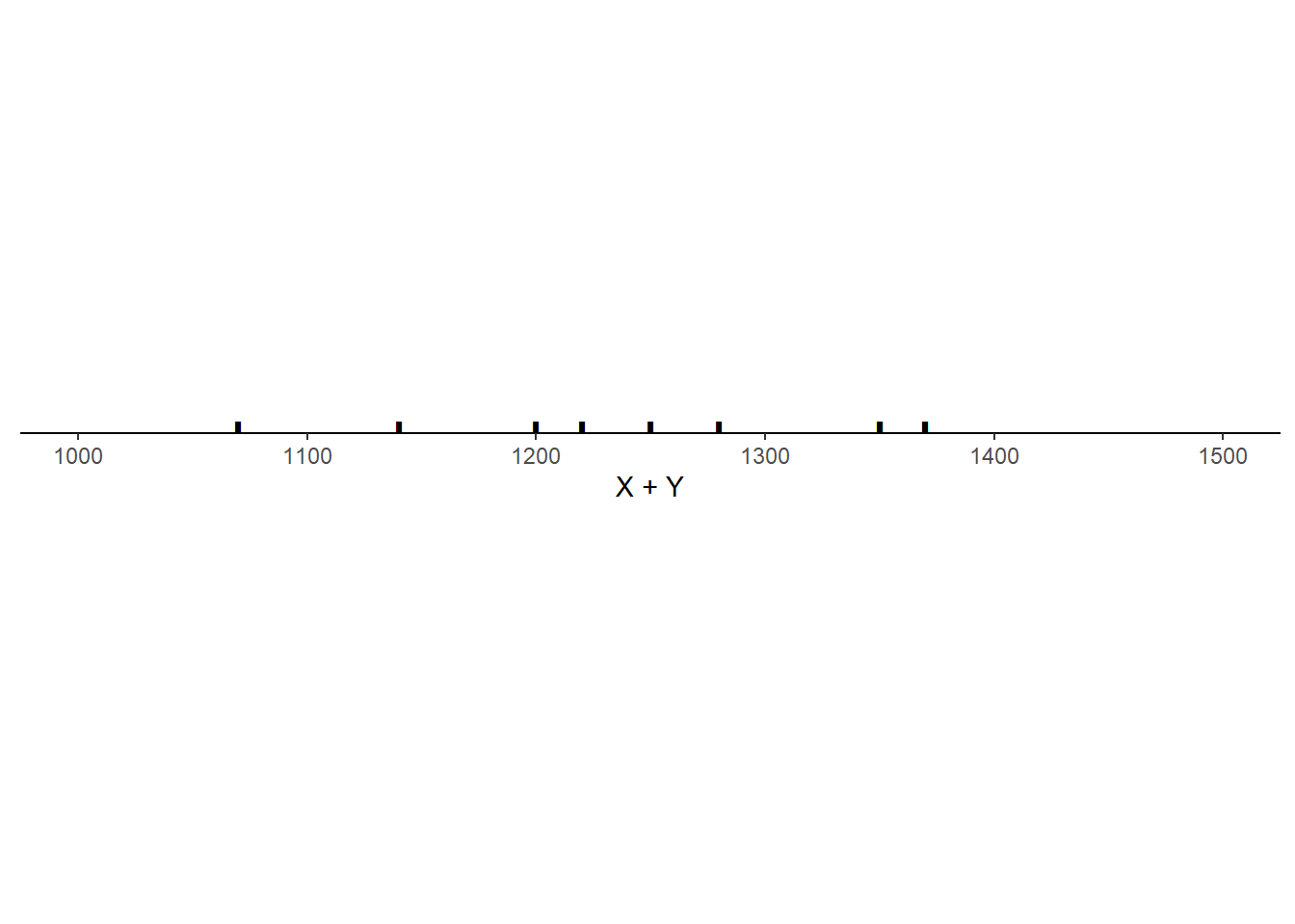
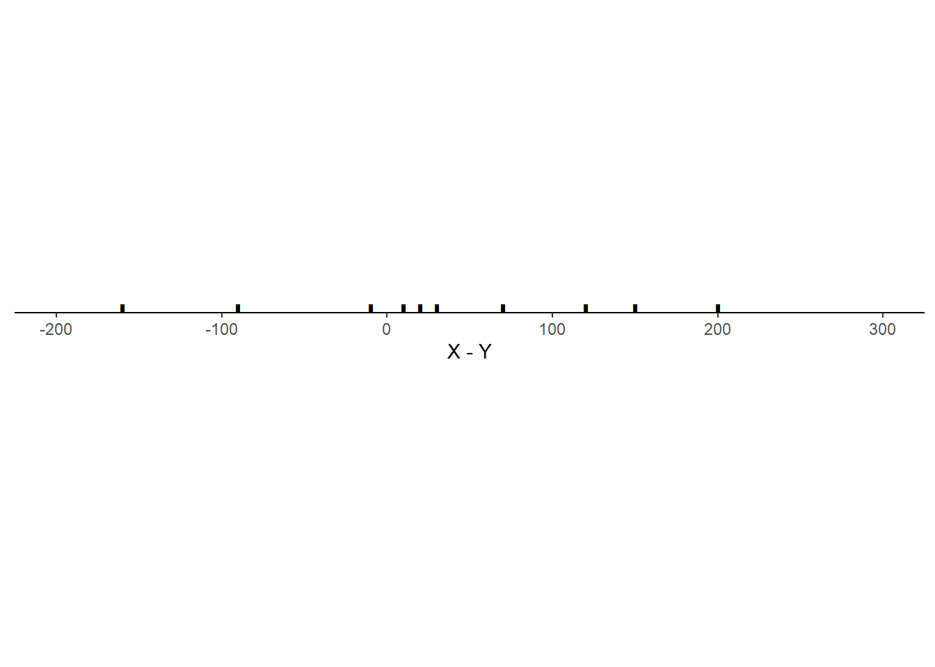
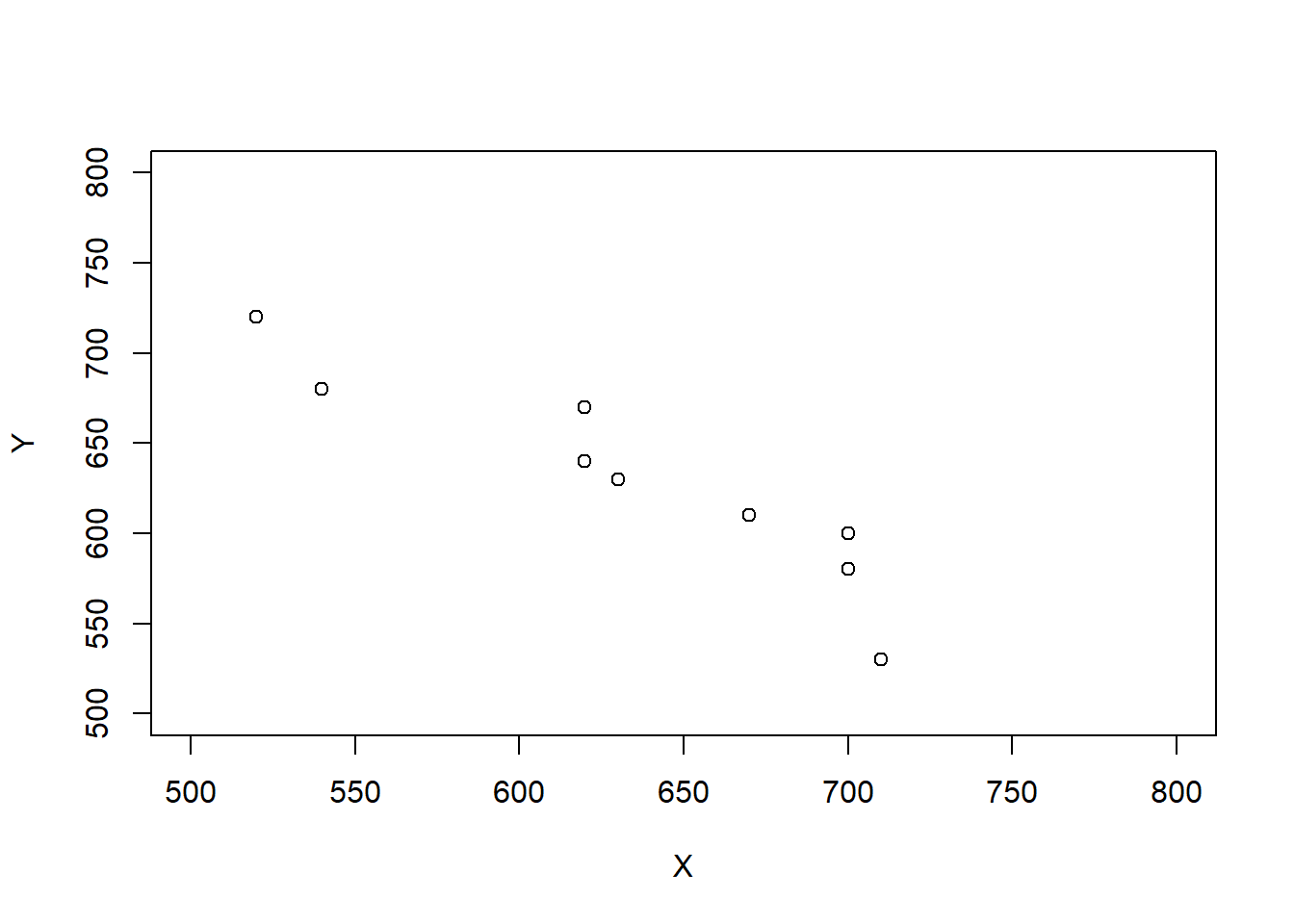
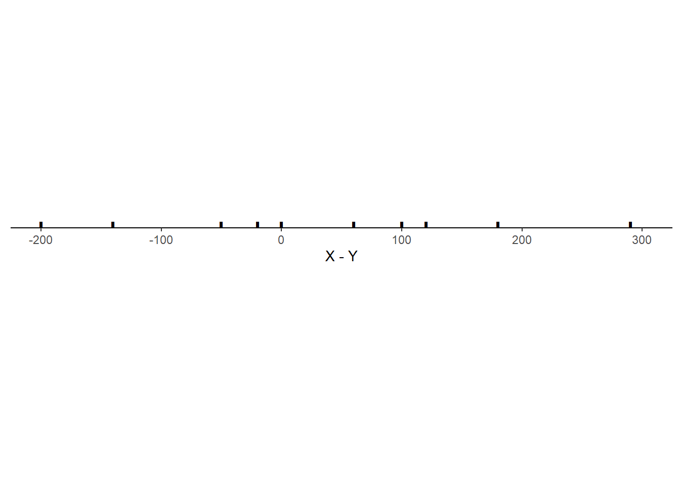
Example 5.29 Consider the three scenarios depicted in the tables and plots below. Each scenario contains SAT Math (\(X\)) and Reading (\(Y\)) scores for 10 hypothetical students, along with the total score (\(T = X + Y\)) and the difference between the Math and Reading scores (\(D = X - Y\), negative values indicate lower Math than Reading scores). Note that the 10 \(X\) values are the same in each scenario, and the 10 \(Y\) values are the same in each scenario, but the \((X, Y)\) values are paired in different ways: the correlation130 is 0.78 in scenario 1, -0.02 in scenario 2, and -0.94 in scenario 3.
- What is the mean of \(T = X + Y\) in each scenario? How does it relate to the means of \(X\) and \(Y\)? Does the correlation affect the mean of \(T = X + Y\)?
- What is the mean of \(D = X - Y\) in each scenario? How does it relate to the means of \(X\) and \(Y\)? Does the correlation affect the mean of \(D = X - Y\)?
Scenario 1.
| Student | \(X\) | \(Y\) | \(T\) | \(D\) |
|---|---|---|---|---|
| 1 | 520 | 530 | 1050 | -10 |
| 2 | 540 | 470 | 1010 | 70 |
| 3 | 620 | 670 | 1290 | -50 |
| 4 | 620 | 630 | 1250 | -10 |
| 5 | 630 | 600 | 1230 | 30 |
| 6 | 670 | 610 | 1280 | 60 |
| 7 | 700 | 680 | 1380 | 20 |
| 8 | 700 | 580 | 1280 | 120 |
| 9 | 710 | 640 | 1350 | 70 |
| 10 | 760 | 720 | 1480 | 40 |
| Mean | 647 | 613 | 1260 | 34 |
| SD | 72 | 70 | 134 | 47 |
| Corr(\(X\), \(Y\)) | 0.78 |
Scenario 2.
| Student | \(X\) | \(Y\) | \(T\) | \(D\) |
|---|---|---|---|---|
| 1 | 520 | 680 | 1200 | -160 |
| 2 | 540 | 530 | 1070 | 10 |
| 3 | 620 | 630 | 1250 | -10 |
| 4 | 620 | 600 | 1220 | 20 |
| 5 | 630 | 720 | 1350 | -90 |
| 6 | 670 | 470 | 1140 | 200 |
| 7 | 700 | 670 | 1370 | 30 |
| 8 | 700 | 580 | 1280 | 120 |
| 9 | 710 | 640 | 1350 | 70 |
| 10 | 760 | 610 | 1370 | 150 |
| Mean | 647 | 613 | 1260 | 34 |
| SD | 72 | 70 | 98 | 103 |
| Corr(\(X\), \(Y\)) | -0.04 |
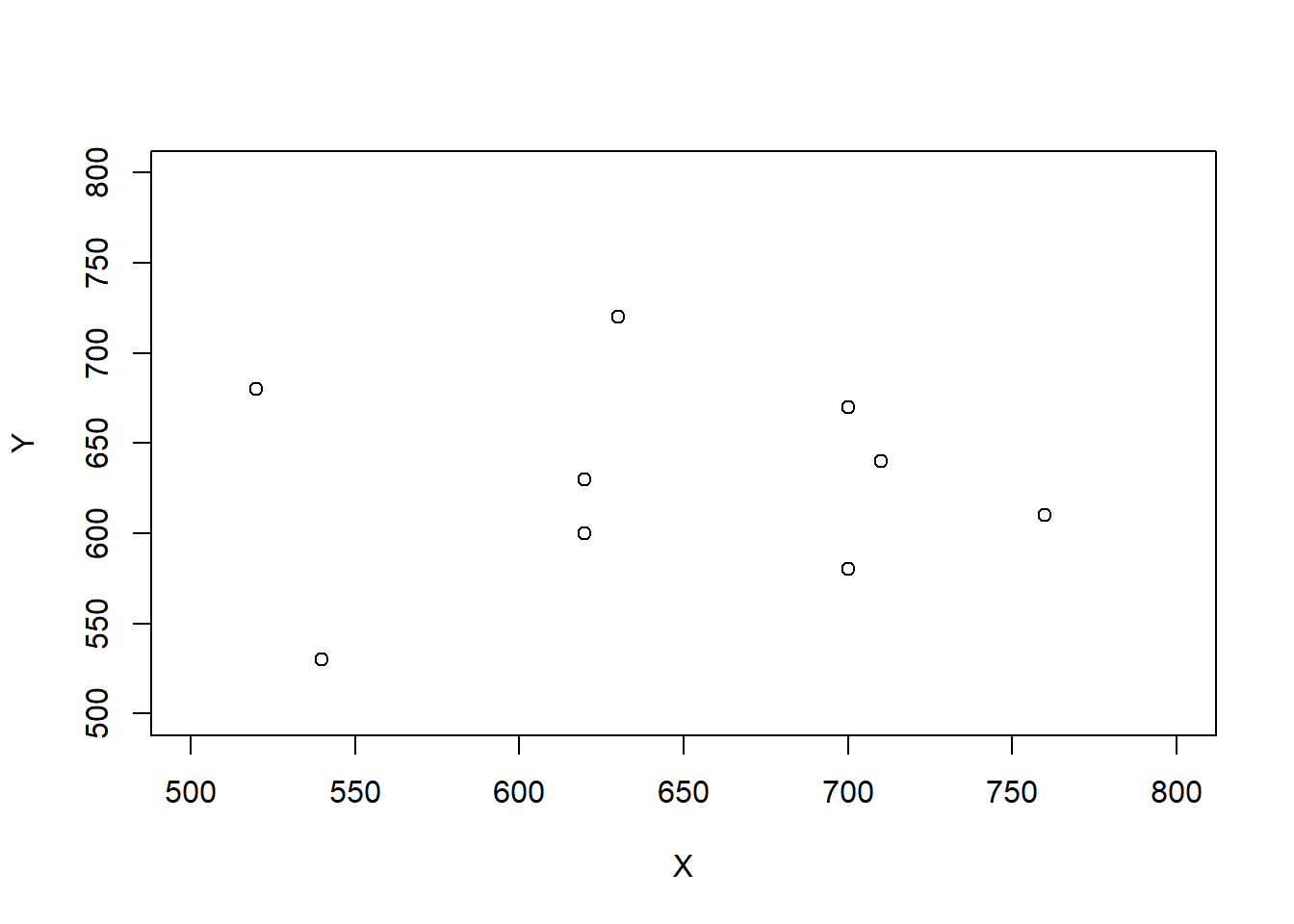
Scenario 3.
| Student | \(X\) | \(Y\) | \(T\) | \(D\) |
|---|---|---|---|---|
| 1 | 520 | 720 | 1240 | -200 |
| 2 | 540 | 680 | 1220 | -140 |
| 3 | 620 | 670 | 1290 | -50 |
| 4 | 620 | 640 | 1260 | -20 |
| 5 | 630 | 630 | 1260 | 0 |
| 6 | 670 | 610 | 1280 | 60 |
| 7 | 700 | 600 | 1300 | 100 |
| 8 | 700 | 580 | 1280 | 120 |
| 9 | 710 | 530 | 1240 | 180 |
| 10 | 760 | 470 | 1230 | 290 |
| Mean | 647 | 613 | 1260 | 34 |
| SD | 72 | 70 | 26 | 140 |
| Corr(\(X\), \(Y\)) | -0.94 |

Solution. to Example 5.29
Show/hide solution
- In each situation, the mean of \(X+Y\) is \(1260 = 647 + 613\), which is equal to the sum of the means of \(X\) and \(Y\). Even though the joint distribution of \((X, Y)\) pairs and the distribution of the sum \(X+Y\) are different for each situation, the correlation between \(X\) and \(Y\) does not affect the average of the \(X + Y\).
- In each situation, the mean of \(X-Y\) is \(1260 = 647 - 613 = 34\), which is equal to the difference of the means of \(X\) and \(Y\). Even though the joint distribution of \((X, Y)\) pairs and the distribution of the difference \(X-Y\) are different for each situation, the correlation between \(X\) and \(Y\) does not affect the average of the \(X - Y\).
Linearity of expected value. For any two random variables \(X\) and \(Y\), \[\begin{align*} \textrm{E}(X + Y) & = \textrm{E}(X) + \textrm{E}(Y) \end{align*}\] That is, the expected value of the sum is the sum of expected values, regardless of how the random variables are related. Therefore, you only need to know the marginal distributions of \(X\) and \(Y\) to find the expected value of their sum. (But keep in mind that the distribution of \(X+Y\) will depend on the joint distribution of \(X\) and \(Y\).)
Linearity of expected value follows from simple arithmetic properties of numbers. Whether in the short run or the long run, \[\begin{align*} \text{Average of $X + Y$ } & = \text{Average of $X$} + \text{Average of $Y$} \end{align*}\] regardless of the joint distribution of \(X\) and \(Y\). For example, for the two \((X, Y)\) pairs (4, 3) and (2, 1) \[ \text{Average of $X + Y$ } = \frac{(4+3)+(2+1)}{2} = \frac{4+2}{2} + \frac{3+1}{2} = \text{Average of $X$} + \text{Average of $Y$}. \] Changing the \((X, Y)\) pairs to (4, 1) and (2, 3) only moves values around in the calculation of the average without affecting the result. \[ \text{Average of $X + Y$ } = \frac{(4+1)+(2+3)}{2} = \frac{4+2}{2} + \frac{3+1}{2} = \text{Average of $X$} + \text{Average of $Y$}. \]
A linear combination of two random variables \(X\) and \(Y\) is of the form \(aX + bY\) where \(a\) and \(b\) are non-random constants. Combining properties of linear rescaling with linearity of expected value yields the expected value of a linear combination. \[ \textrm{E}(aX + bY) = a\textrm{E}(X)+b\textrm{E}(Y) \] For example, \(\textrm{E}(X - Y) = \textrm{E}(X) - \textrm{E}(Y)\). The left side above, \(\textrm{E}(aX+bY)\), represents the “long way”: find the distribution of \(aX + bY\), which will depend on the joint distribution of \(X\) and \(Y\), and then use the definition of expected value. The right side above, \(a\textrm{E}(X)+b\textrm{E}(Y)\), is the “short way”: find the expected values of \(X\) and \(Y\), which only requires their marginal distributions, and plug those numbers into the transformation formula. Similar to LOTUS, linearity of expected value provides a way to find the expected value of certain random variables without first finding the distribution of the random variables.
Linearity of expected value extends naturally to more than two random variables.
Example 5.30 Recall the matching problem in Example 5.1. We showed that the expected value of the number of matches \(X\) is \(\textrm{E}(X)=1\) when \(n=4\). Now consider a general \(n\): there are \(n\) objects that are shuffled and placed uniformly at random in \(n\) spots with one object per spot. Let \(X\) be the number of matches. Can you find a general formula for \(\textrm{E}(X)\)?
- Before proceeding take a minute to consider: how do you think \(\textrm{E}(X)\) depends on \(n\)? Will \(\textrm{E}(X)\) increase as \(n\) increases? Decrease? Stay the same?
- When \(n=4\) we derived the distribution of \(X\) and used it to find \(\textrm{E}(X)=1\). Now we’ll see how to find \(\textrm{E}(X)\) without first finding the distribution of \(X\). The key is to use the indicator random variables from Example 2.11. Let \(\textrm{I}_1\) be the indicator that object 1 is placed correctly in spot 1. Find \(\textrm{E}(\textrm{I}_1)\).
- When \(n=4\), find \(\textrm{E}(\textrm{I}_j)\) for \(j=1,2,3, 4\).
- What is the relationship between the random variables \(X\) and \(\textrm{I}_1, \textrm{I}_2,\textrm{I}_3, \textrm{I}_4\)?
- Use the previous parts to find \(\textrm{E}(X)\).
- Now consider a general \(n\). Let \(\textrm{I}_i\) be the indicator that object \(j\) is placed correctly in spot \(j\), \(j=1, \ldots, n\). Find \(\textrm{E}(\textrm{I}_j)\).
- What is the relationship between \(X\) and \(\textrm{I}_1, \ldots, \textrm{I}_n\)?
- Find \(\textrm{E}(X)\). Be amazed.
- Interpret \(\textrm{E}(X)\) is context.
Show/hide solution
- There are two common guesses. (1) As \(n\) increases, there are more chances for a match, so maybe \(\textrm{E}(X)\) increases with \(n\). (2) But as \(n\) increases the chance that any particular object goes in the correct spot decreases, so maybe \(\textrm{E}(X)\) decreases with \(n\). These considerations move \(\textrm{E}(X)\) in opposite directions; how do they balance?
- Recall that the expected value of an indicator random variable is just the probability of the corresponding event. There are \(4\) objects which are equally likely to be placed in spot 1, only 1 of which is correct. The probability that object 1 is correctly placed in spot 1 is \(1/4\). That is, \(\textrm{E}(\textrm{I}_1) = (1)(1/4) + (0)(1 - 1/4) = 1/4\).
- If the objects are placed uniformly at random then no object is more or less likely than any other to be placed in its correct spot, so the probability and expected value should be the same for all \(j\). Given any spot \(j\), any of the \(4\) objects is equally likely to be placed in spot \(j\), and only one of those is the correct object, so \(\textrm{P}(\textrm{I}_j = 1) = 1/4\), and \(\textrm{E}(\textrm{I}_j) = 1/4\). Note that these are marginal probabilities and marginal expected values; see the note after the example below.
- Recall Example 2.11. We can count the total number of matches by starting with a count of 0, inspecting each spot, and incrementally adding 1 to our counter each time object \(j\) matches spot \(j\) for \(j=1, \ldots, 4\). That is, the total number of matches is the sum of the indicator random variables: \(X=\textrm{I}_1 + \textrm{I}_2+\textrm{I}_3+\textrm{I}_4\).
- Linearity of expected value says the expected value of the sum is the sum of the expected values \[\begin{align*} \textrm{E}(X) & = \textrm{E}(\textrm{I}_1 + \textrm{I}_2 + \textrm{I}_3 + \textrm{I}_4)\\ & = \textrm{E}(\textrm{I}_1) + \textrm{E}(\textrm{I}_2) + \textrm{E}(\textrm{I}_3) + \textrm{E}(\textrm{I}_4)\\ & = 1/4 + 1/4 + 1/4 + 1/4\\ & = 4(1/4) = 1 \end{align*}\]
- Now we repeat the above process for a general \(n\). If the objects are placed uniformly at random then no object is more or less likely than any other to be placed in its correct spot, so the probability and expected value should be the same for all \(j=1, \ldots, n\). Given any spot \(j\), any of the \(n\) objects is equally likely to be placed in spot \(j\), and only one of those is the correct object, so \(\textrm{P}(\textrm{I}_j = 1) = 1/n\), and \(\textrm{E}(I_j) = 1/n\).
- We can count the total number of matches by incrementally adding 1 to our counter each time object \(j\) matches spot \(j\) for \(j=1, \ldots, n\). That is, the total number of matches is the sum of the indicator random variables: \(X=\textrm{I}_1 + \cdots + \textrm{I}_n\).
- Use linearity of expected value \[\begin{align*} \textrm{E}(X) & = \textrm{E}(\textrm{I}_1 + \textrm{I}_2 + \cdots + \textrm{I}_n)\\ & = \textrm{E}(\textrm{I}_1) + \textrm{E}(\textrm{I}_2) + \cdots + \textrm{E}(\textrm{I}_n)\\ & = \frac{1}{n} + \frac{1}{n} + \cdots + \frac{1}{n}\\ & = n\left(\frac{1}{n}\right) = 1 \end{align*}\] Regardless of the value of \(n\), \(\textrm{E}(X) = 1\)!
- Imagine placing \(n\) distinct objects uniformly at random in \(n\) distinct spots with one object per spot. Then over many such placements, on average 1 object per placement is placed in the correct spot regardless of the number of objects/spots.
The answer to the previous problem is not an approximation: the expected value of the number of matches is equal to 1 for any \(n\). We think that’s pretty amazing. (We’ll see some even more amazing results for this problem later.) Notice that we computed the expected value without first finding the distribution of \(X\). When \(n=4\) we found the distribution of \(X\) by enumerating all the possibilities. Obviously this is not feasible when \(n\) is large, and in general it is difficult to find the exact distribution of \(X\) in the matching problem (though we’ll see a pretty good approximation later). However, as the previous example shows, we don’t need to find the distribution of \(X\) to find \(\textrm{E}(X)\).
Intuitively, if the objects are placed in the spots uniformly at random, then the probability that object \(j\) is placed in the correct spot should be the same for all the objects, \(1/n\). But you might have said: “if object 1 goes in spot 1, there are only \(n-1\) objects that can go in spot 2, so the probability that object 2 goes in spot to is \(1/(n-1)\)”. That is true if object 1 goes in spot 1. However, when computing the marginal probability that object 2 goes in spot 2, we don’t know whether object 1 went in spot 1 or not, so the probability needs to account for both cases. Remember, there is a difference between marginal/unconditional probability and conditional probability; recall Section 3.4. Linearity of expected value is useful because we only need the marginal distribution of each random variable to compute the sum of their expected values.
When a problem asks “find the expected number of…” it’s a good idea to try using indicator random variables and linearity of expected value. The following is a general statement of the strategy we used in the matching problem.
Let \(A_1, A_2, \ldots, A_n\) be a collection of \(n\) events. Suppose event \(i\) occurs with marginal probability \(p_i=\textrm{P}(A_i)\). Let \(N = \textrm{I}_{A_i} + \textrm{I}_{A_2} + \cdots + \textrm{I}_{A_n}\) be the random variable which counts the number of the events in the collection which occur. Then the expected number of events that occur is the sum of the event probabilities. \[ \textrm{E}(N) = \sum_{i=1}^n p_i. \] If each event has the same probability, \(p_i \equiv p\), then \(\textrm{E}(N)\) is equal to \(np\). These formulas for the expected number of events are true regardless of whether there is any association between the events (that is, regardless of whether the events are independent.)
For example, in the matching problem \(A_i\) was the event that object \(i\) was placed in spot \(i\) and \(p_i=1/n\) for all \(i\).
Example 5.31 Kids wake up during the night. On any given night,
- the probability that Paul wakes up is 1/14
- the probability that Bob wakes up is 2/7
- the probability that Tommy wakes up is 1/30
- the probability that Chris wakes up is 1/2
- the probability that Slim wakes up is 6/7.
If any kid wakes up they’re likely to wake other kids up too. Find and interpret the expected number of kids that wake up on any given night.
Show/hide solution
Simply add the probabilities: \(1/14 + 2/7 + 1/30+ 1/2 + 6/7=1.75\). The expected number of kids to wake up in a night is 1.75. Over many nights, on average 1.75 kids wake up per night.
The fact that kids wake each other up implies that the events are not independent, but this is irrelevant here. Because of linearity of expected value, we only need to know the marginal probability131 of each event (provided) in order to determine the expected number of events occur. (The distribution of the number of kids that wake up would depend the relationships between the events, but not the long run average value.)
When computing the expected value of a random variable, consider if it can be written as a sum of component random variables. If so, then using linearity of expected value is usually easier than first finding the distribution of the random variable. Of course, the expected value is only one feature of the distribution of a random variable; there is much more to a distribution than its expected value.
5.5.3 Variance of linear combinations of random variables
We have seen that correlation does not affect the expected value of a linear combination of random variables. But what affect, if any, does correlation have on the variance of a linear combination of random variables?
Example 5.32 Consider a random variable \(X\) with \(\textrm{Var}(X)=1\). What is \(\textrm{Var}(2X)\)?
- Walt says: \(\textrm{SD}(2X) = 2\textrm{SD}(X)\) so \(\textrm{Var}(2X) = 2^2\textrm{Var}(X) = 4(1) = 4\).
- Jesse says: Variance of a sum is a sum of variances, so \(\textrm{Var}(2X) = \textrm{Var}(X+X)\) which is equal to \(\textrm{Var}(X)+\textrm{Var}(X) = 1+1=2\).
Who is correct? Why is the other wrong?
Show/hide solution
If \(\textrm{Var}(X)=1\) then \(\textrm{Var}(2X)= 4\). Walt is correctly using properties of linear rescaling. Jesse is assuming that a variance of a sum is the sum of the variances, which is not true in general. We’ll see why below.
When two variables are correlated the degree of the association will affect the variability of linear combinations of the two variables.
Example 5.33 Recall Example 5.29.
- In which of the three scenarios is \(\textrm{Var}(X + Y)\) the largest? Can you explain why?
- In which of the three scenarios is \(\textrm{Var}(X + Y)\) the smallest? Can you explain why?
- In which scenario is \(\textrm{Var}(X + Y)\) roughly equal to the sum of \(\textrm{Var}(X)\) and \(\textrm{Var}(Y)\)?
- In which of the three scenarios is \(\textrm{Var}(X - Y)\) the largest? Can you explain why?
- In which of the three scenarios is \(\textrm{Var}(X - Y)\) the smallest? Can you explain why?
- In which scenario is \(\textrm{Var}(X - Y)\) roughly equal to the sum of \(\textrm{Var}(X)\) and \(\textrm{Var}(Y)\)?
Solution. to Example 5.33
Show/hide solution
- Variance of \(X + Y\) is largest when \(\textrm{Corr}(X, Y)\) is near 1 (scenario 1). With a strong positive correlation, students who scored high on Math tended to also score high on Reading so their total score was very high; students who scored low on Math tended to also score low on Reading so their total score was very low. Of these three scenarios we see the most variability in \(X+Y\) in scenario 1.
- Variance of \(X + Y\) is smallest when \(\textrm{Corr}(X, Y)\) is near \(-1\) (scenario 3). With a strong negative correlation, students who scored high on Math tended to score low on Reading so their total score was moderate; students who scored low on Math tended to score high on Reading so their total score was moderate. Of these three scenarios we see the least variability in \(X+Y\) in scenario 3.
- When the correlation between \(X\) and \(Y\) is near 0 (scenario 2) the variance of \(X + Y\) is roughly equal to the sum of the variances.
- Variance of \(X - Y\) is largest when \(\textrm{Corr}(X, Y)\) is near \(-1\) (scenario 3). With a strong negative correlation, students who scored high on Math tended to score low on Reading so their difference in scores was high and positive; students who scored low on Math tended to score high on Reading so their difference in scores was high and negative. Of these three scenarios we see the most variability in \(X-Y\) in scenario 3.
- Variance of \(X - Y\) is smallest when \(\textrm{Corr}(X, Y)\) is near 1 (scenario 1). With a strong positive correlation, students who scored high on Math tended to also score high on Reading so their difference in scores was small; students who scored low on Math tended to also score low on Reading so their difference in scores was small. Of these three scenarios we see the least variability in \(X-Y\) in scenario 1.
- When the correlation between \(X\) and \(Y\) is near 0 (scenario 2) the variance of \(X - Y\) is roughly equal to the sum of the variances. That is, when the correlation is 0, the sum \(X+Y\) and the difference \(X-Y\) have the same variance.
The degree of correlation between two random variables affects the variability of their sum and difference. The following formulas represent the math behind the observations we made in the previous problem.
Variance of sums and differences of random variables. \[\begin{align*} \textrm{Var}(X + Y) & = \textrm{Var}(X) + \textrm{Var}(Y) + 2\textrm{Cov}(X, Y)\\ \textrm{Var}(X - Y) & = \textrm{Var}(X) + \textrm{Var}(Y) - 2\textrm{Cov}(X, Y) \end{align*}\]
The left side represents first finding the distribution of the random variable \(X+Y\) and computing its variance. The right side represents using the joint (and marginal) distribution of \((X, Y)\) to compute the variance of the sum. However, to compute the right side we do not need the full joint and marginal distributions; we simply need the marginal variances and the covariance (or correlation).
Example 5.34 Assume that SAT Math (\(X\)) and Reading (\(Y\)) scores follow a Bivariate Normal distribution, Math scores have mean 527 and standard deviation 107, and Reading scores have mean 533 and standard deviation 100. Compute \(\textrm{Var}(X + Y)\) and \(\textrm{SD}(X+Y)\) for each of the following correlations.
- \(\textrm{Corr}(X, Y) = 0.77\)
- \(\textrm{Corr}(X, Y) = 0.40\)
- \(\textrm{Corr}(X, Y) = 0\)
- \(\textrm{Corr}(X, Y) = -0.77\)
Show/hide solution
Recall that we can obtain covariance from correlation: \(\textrm{Cov}(X, Y) = \textrm{Corr}(X, Y)\textrm{SD}(X)\textrm{SD}(Y) = (0.77)(107)(100) = 8239\).
- \(\textrm{Var}(X + Y) = \textrm{Var}(X) + \textrm{Var}(Y) + 2\textrm{Cov}(X, Y) = 107^2 + 100^2 + 2(8239)=37927\). \(\textrm{SD}(X+Y)=\sqrt{37927} = 195\).
- \(\textrm{Var}(X + Y) = 107^2 + 100^2 + 2(0.40)(107)(100)=30009\). \(\textrm{SD}(X+Y)= 173\).
- \(\textrm{Var}(X + Y) = 107^2 + 100^2 + 0=21449\). \(\textrm{SD}(X+Y)= 146\).
- \(\textrm{Var}(X + Y) = 107^2 + 100^2 + 2(-0.77)(107)(100)=4971\). \(\textrm{SD}(X+Y)= 70\).
If \(X\) and \(Y\) have a positive correlation: Large values of \(X\) are associated with large values of \(Y\) so the sum is really large, and small values of \(X\) are associated with small values of \(Y\) so the sum is really small. That is, the sum exhibits more variability than it would if the values of \(X\) and \(Y\) were uncorrelated.
If \(X\) and \(Y\) have a negative correlation: Large values of \(X\) are associated with small values of \(Y\) so the sum is moderate, and small values of \(X\) are associated with large values of \(Y\) so the sum is moderate. That is, the sum exhibits less variability than it would if the values of \(X\) and \(Y\) were uncorrelated.
The following simulation illustrates the previous example when the correlation is 0.77. First we simulate \((X, Y)\) pairs.
X, Y = RV(BivariateNormal(mean1 = 527, sd1 = 107, mean2 = 533, sd2 = 100, corr = 0.77))

x_and_y = (X & Y).sim(10000)

x_and_y| Index | Result |
|---|---|
| 0 | (455.2602024501872, 486.3128592188935) |
| 1 | (494.9350534575873, 523.4888776432035) |
| 2 | (403.0585932211548, 546.0277243747076) |
| 3 | (495.2751204852371, 457.81848440739554) |
| 4 | (441.50980401769175, 385.89681129821486) |
| 5 | (622.1345875746758, 514.1400956487747) |
| 6 | (462.2997400177747, 411.934401977255) |
| 7 | (382.02244445876556, 389.8744908339503) |
| 8 | (405.6935289929199, 540.2619032076933) |
| ... | ... |
| 9999 | (574.8101926840565, 482.5589557618666) |
x_and_y.plot()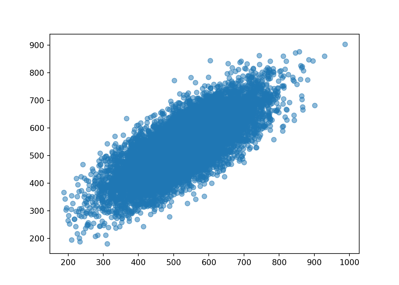
x_and_y.mean()## (528.2341445704116, 533.8553991883414)x_and_y.var()## (11482.11401247682, 9895.96501690312)x_and_y.sd()## (107.15462664988769, 99.47846509121017)Now we look at the sum \(X + Y\).
So that our simulation results our consistent with those above we’ll define x + y in “simulation world” (but we could have defined X + Y in “random variable world” and then simulated values of it.)
x = x_and_y[0]
y = x_and_y[1]

t = x + y

t| Index | Result |
|---|---|
| 0 | 941.5730616690807 |
| 1 | 1018.4239311007908 |
| 2 | 949.0863175958625 |
| 3 | 953.0936048926326 |
| 4 | 827.4066153159066 |
| 5 | 1136.2746832234507 |
| 6 | 874.2341419950296 |
| 7 | 771.8969352927159 |
| 8 | 945.9554322006131 |
| ... | ... |
| 9999 | 1057.3691484459232 |
t.plot()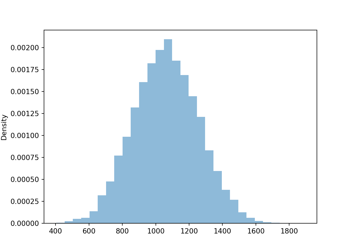
The simulated mean, variance, and standard deviation as close to what we computed in the previous example (of course, there is natural simulation variability).
t.mean()## 1062.0895437587512t.var()## 37750.71994001943t.sd()## 194.29544498011123Now we compare the distribution of the sum for each of the four cases for the correlation. Notice how the variability of \(X+Y\) changes based on the correlation. The variability of \(X + Y\) is largest when the correlation is strong and positive, and smallest when the correlation is strong and negative.
X2, Y2 = RV(BivariateNormal(mean1 = 527, sd1 = 107, mean2 = 533, sd2 = 100, corr = 0.4))
t2 = (X2 + Y2).sim(10000)

X3, Y3 = RV(BivariateNormal(mean1 = 527, sd1 = 107, mean2 = 533, sd2 = 100, corr = 0))
t3 = (X3 + Y3).sim(10000)

X4, Y4 = RV(BivariateNormal(mean1 = 527, sd1 = 107, mean2 = 533, sd2 = 100, corr = -0.77))
t4 = (X4 + Y4).sim(10000)

plt.figure()
t.plot()
t2.plot()
t3.plot()
t4.plot()

plt.legend(['corr = 0.77', 'corr = 0.40', 'corr = 0', 'corr = -0.77']);
plt.show()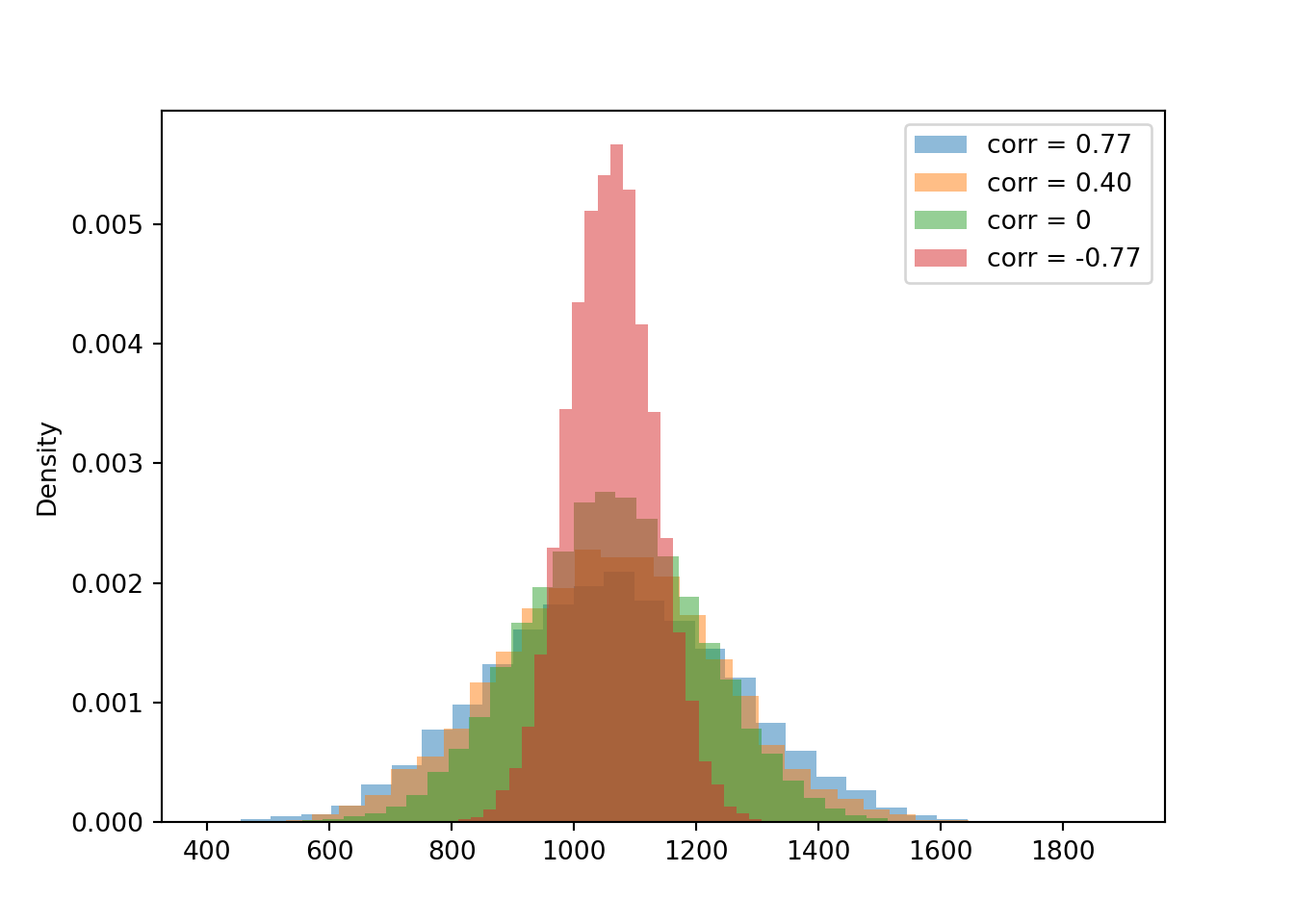
The simulated means, variances, and standard deviations as close to what we computed in the previous example (of course, there is natural simulation variability).
t.mean(), t2.mean(), t3.mean(), t4.mean()## (1062.0895437587512, 1057.7149069494524, 1062.7173511993979, 1060.8279487502857)t.sd(), t2.sd(), t3.sd(), t4.sd()## (194.29544498011123, 175.2109269618061, 144.8840860894233, 70.76216620676561)Compare the 90th percentiles of \(X+Y\). The largest value for the 90th percentile occurs when there is the most variability in the sum, so we see more extreme values of the sum.
t.quantile(0.9), t2.quantile(0.9), t3.quantile(0.9), t4.quantile(0.9)## (1312.6150384985604, 1278.7121641435522, 1249.51979995194, 1151.3615819594868)Example 5.35 Continuing the previous example. Compute \(\textrm{Var}(X - Y)\) and \(\textrm{SD}(X-Y)\) for each of the following correlations.
- \(\textrm{Corr}(X, Y) = 0.77\)
- \(\textrm{Corr}(X, Y) = 0.40\)
- \(\textrm{Corr}(X, Y) = 0\)
- \(\textrm{Corr}(X, Y) = -0.77\)
Show/hide solution
- \(\textrm{Cov}(X, Y) = \textrm{Corr}(X, Y)\textrm{SD}(X)\textrm{SD}(Y) = (0.77)(107)(100) = 8239\). \(\textrm{Var}(X - Y) = \textrm{Var}(X) + \textrm{Var}(Y) - 2\textrm{Cov}(X, Y) = 107^2 + 100^2 - 2(8239)=4971\). \(\textrm{SD}(X-Y)=\sqrt{4971} = 70\).
- \(\textrm{Var}(X - Y) = 107^2 + 100^2 - 2(0.40)(107)(100)=12889\). \(\textrm{SD}(X-Y)= 114\).
- \(\textrm{Var}(X - Y) = 107^2 + 100^2 - 0=21449\). \(\textrm{SD}(X-Y)= 146\).
- \(\textrm{Var}(X - Y) = 107^2 + 100^2 - 2(-0.77)(107)(100)=37927\). \(\textrm{SD}(X-Y)= 195\).
If \(X\) and \(Y\) have a positive correlation: Large values of \(X\) are associated with large values of \(Y\) so the difference is small, and small values of \(X\) are associated with small values of \(Y\) so the difference is small. That is, the difference exhibits less variability than it would if the values of \(X\) and \(Y\) were uncorrelated.
If \(X\) and \(Y\) have a negative correlation: Large values of \(X\) are associated with small values of \(Y\) so the difference is large and positive, and small values of \(X\) are associated with large values of \(Y\) so the difference is large and negative. That is, the difference exhibits more variability than it would if the values of \(X\) and \(Y\) were uncorrelated.
We continue the simulation from above when the correlation is 0.77.
New we look at the difference \(X - Y\).
Again, we define the difference x - y in “simulation world” (but we could have defined X - Y in “random variable world” and then simulated values of it).
d = x - y

d| Index | Result |
|---|---|
| 0 | -31.0526567687063 |
| 1 | -28.553824185616236 |
| 2 | -142.96913115355284 |
| 3 | 37.45663607784155 |
| 4 | 55.61299271947689 |
| 5 | 107.99449192590112 |
| 6 | 50.3653380405197 |
| 7 | -7.852046375184727 |
| 8 | -134.56837421477343 |
| ... | ... |
| 9999 | 92.25123692218983 |
d.plot()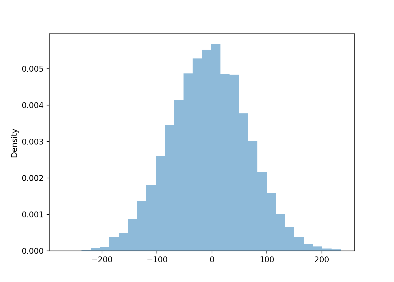
Now we compare the distributions of the difference \(X - Y\) for each of the four cases of correlation. Notice how the variability of \(X-Y\) changes based on the correlation. The variability of \(X - Y\) is largest when the correlation is strong and negative, and smallest when the correlation is strong and positive.
X2, Y2 = RV(BivariateNormal(mean1 = 527, sd1 = 107, mean2 = 533, sd2 = 100, corr = 0.4))
d2 = (X2 - Y2).sim(10000)

X3, Y3 = RV(BivariateNormal(mean1 = 527, sd1 = 107, mean2 = 533, sd2 = 100, corr = 0))
d3 = (X3 - Y3).sim(10000)

X4, Y4 = RV(BivariateNormal(mean1 = 527, sd1 = 107, mean2 = 533, sd2 = 100, corr = -0.77))
d4 = (X4 - Y4).sim(10000)

plt.figure()
d.plot()
d2.plot()
d3.plot()
d4.plot()

plt.legend(['corr = 0.77', 'corr = 0.40', 'corr = 0', 'corr = -0.77']);
plt.show()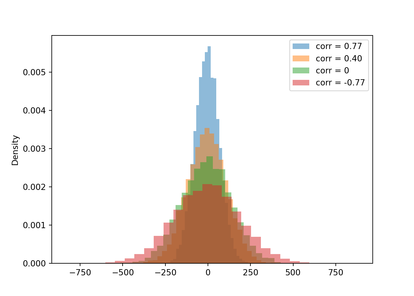
The simulated mean, variance, and standard deviation as close to what we computed in the previous example (of course, there is natural simulation variability).
d.mean(), d2.mean(), d3.mean(), d4.mean()## (-5.621254617931615, -6.638857562084749, -8.04075740476792, -6.051902833122087)d.sd(), d2.sd(), d3.sd(), d4.sd()## (70.74912097503633, 113.64198453486081, 145.1636701458166, 192.80093410624653)Compare the 90th percentiles of \(X-Y\). The largest value for the 90th percentile occurs when there is the most variability in the difference, so we see more extreme values of the difference.
d.quantile(0.9), d2.quantile(0.9), d3.quantile(0.9), d4.quantile(0.9)## (84.97983894245704, 139.0675986579186, 177.83951287654264, 241.12360021005566)The variance of the sum is the sum of the variances if and only if \(X\) and \(Y\) are uncorrelated. \[\begin{align*} \textrm{Var}(X+Y) & = \textrm{Var}(X) + \textrm{Var}(Y)\qquad \text{if $X, Y$ are uncorrelated}\\ \textrm{Var}(X-Y) & = \textrm{Var}(X) + \textrm{Var}(Y)\qquad \text{if $X, Y$ are uncorrelated} \end{align*}\]
The variance of the difference of uncorrelated random variables is the sum of the variances. Think just about the range of values. Suppose SAT Math and Reading scores are each uniformly distributed on the interval [200, 800]. Then the sum takes values in [400, 1600], an interval of length 1200. The difference takes values in \([-600, 600]\), also an interval of length 1200.
Combining the formula for variance of sums with some properties of covariance in the next subsection, we have a general formula for the variance of a linear combination of two random variables. If \(a, b, c\) are non-random constants and \(X\) and \(Y\) are random variables then \[ \textrm{Var}(aX + bY + c) = a^2\textrm{Var}(X) + b^2\textrm{Var}(Y) + 2ab\textrm{Cov}(X, Y) \]
5.5.4 Bilinearity of covariance
The formulas for variance of sums and differences are application of several more general properties of covariance. Let \(X,Y,U,V\) be random variables and \(a,b,c,d\) be non-random constants.
Properties of covariance. \[\begin{align*} \textrm{Cov}(X, X) &= \textrm{Var}(X)\qquad\qquad\\ \textrm{Cov}(X, Y) & = \textrm{Cov}(Y, X)\\ \textrm{Cov}(X, c) & = 0 \\ \textrm{Cov}(aX+b, cY+d) & = ac\textrm{Cov}(X,Y)\\ \textrm{Cov}(X+Y,\; U+V) & = \textrm{Cov}(X, U)+\textrm{Cov}(X, V) + \textrm{Cov}(Y, U) + \textrm{Cov}(Y, V) \end{align*}\]
- The variance of a random variable is the covariance of the random variable with itself.
- Non-random constants don’t vary, so they can’t co-vary.
- Adding non-random constants shifts the center of the joint distribution but does not affect variability.
- Multiplying by non-random constants changes the scale and hence changes the degree of variability.
- The last property is like a “FOIL” (first, outer, inner, last) property.
The last two properties together are called bilinearity of covariance. These properties extend naturally to sums involving more than two random variables. To compute the covariance between two sums of random variables, compute the covariance between each component random variable in the first sum and each component random variable in the second sum, and sum the covariances of the components.
Example 5.36 Let \(X\) be the number of two-point field goals a basketball player makes in a game, \(Y\) the number of three point field goals made, and \(Z\) the number of free throws made (worth one point each). Assume \(X\), \(Y\), \(Z\) have standard deviations of 2.5, 3.7, 1.8, respectively, and \(\textrm{Corr}(X,Y) = 0.1\), \(\textrm{Corr}(X, Z) = 0.3\), \(\textrm{Corr}(Y,Z) = -0.5\).
- Find the standard deviation of the number of fields goals in a game (not including free throws)
- Find the standard deviation of total points scored on fields goals in a game (not including free throws)
- Find the standard deviation of total points scored in a game.
Show/hide solution
- We want \(\textrm{SD}(X+Y)\), so we first find \(\textrm{Var}(X + Y)\). We could use the formula for a variance of sums, but we’ll use bilinearity of covariance instead to illustrate how it works, and to motivate part 3. \[\begin{align*} \textrm{Var}(X + Y) & = \textrm{Cov}(X + Y, X + Y)\\ & = \textrm{Cov}(X, X) + \textrm{Cov}(X, Y) + \textrm{Cov}(Y, X) + \textrm{Cov}(Y, Y)\\ & = (2.5^2) + (0.1)(2.5)(3.7) + (0.1)(3.7)(2.5) + 3.7^2 = 21.49 \end{align*}\] So \(\textrm{SD}(X + Y) = 4.67\).
- We want \(\textrm{SD}(2X+3Y)\), so we first find \(\textrm{Var}(2X + 3Y)\). We’ll use bilinearity of covariance again. \[\begin{align*} \textrm{Var}(2X + 3Y) & = \textrm{Cov}(2X + 3Y, 2X + 3Y)\\ & = \textrm{Cov}(2X, 2X) + \textrm{Cov}(2X, 3Y) + \textrm{Cov}(3Y, 2X) + \textrm{Cov}(3Y, 3Y)\\ & = 2^2\textrm{Cov}(X, X) + (2)(3)\textrm{Cov}(X, Y) + (3)(2)\textrm{Cov}(Y, X)+ (3)(3)\textrm{Cov}(Y, Y)\\ & = (2^2)(2.5^2) + (2)(3)(0.1)(2.5)(3.7) + (3)(2)(0.1)(3.7)(2.5) + (3^2)(3.7^2) = 159.31 \end{align*}\] So \(\textrm{SD}(2X + 3Y) = 12.62\).
- We want \(\textrm{SD}(2X+3Y + Z)\), so we first find \(\textrm{Var}(2X + 3Y + Z)\). We’ll use bilinearity of covariance again. Notice how we take the covariance of each term in the sum with each of the others. \[\begin{align*} \textrm{Var}(2X + 3Y + Z) & = \textrm{Cov}(2X + 3Y + Z, 2X + 3Y + Z)\\ & = \textrm{Cov}(2X, 2X) + \textrm{Cov}(2X, 3Y) + \textrm{Cov}(2X, Z) \\ & \quad + \textrm{Cov}(3Y, 2X) + \textrm{Cov}(3Y, 3Y) + \textrm{Cov}(3Y, Z)\\ & \quad + \textrm{Cov}(Z, 2X) + \textrm{Cov}(Z, 3Y) + \textrm{Cov}(Z, Z)\\ & = 2^2\textrm{Cov}(X, X) + (2)(3)\textrm{Cov}(X, Y) + (2)(1)\textrm{Cov}(X, Z)\\ & \quad + (3)(2)\textrm{Cov}(Y, X)+ (3)(3)\textrm{Cov}(Y, Y) + (3)(1)\textrm{Cov}(Y, Z)\\ & \quad + (1)(2)\textrm{Cov}(Z, X)+ (1)(3)\textrm{Cov}(Z, Y) + 1^2\textrm{Cov}(Z, Z)\\ & = (2^2)(2.5^2) + (2)(3)(0.1)(2.5)(3.7) + (2)(1)(0.3)(2.5)(1.8)\\ & \quad + (3)(2)(0.1)(3.7)(2.5) + (3^2)(3.7^2) + (3)(1)(-0.5)(3.7)(1.8)\\ & \quad + (1)(2)(0.3)(1.8)(2.5) + (1)(3)(-0.5)(1.8)(3.7) + 1^2(1.8^2)= 114.72 \end{align*}\] So \(\textrm{SD}(2X + 3Y + Z) = 12.16\).
All averages, including those used to compute variance and covariance, are computed by dividing the appropriate sum by 10.↩︎
If there were too much dependence, then the provided marginal probabilities might not be possible. For example if Slim always wakes up all the other kids, then the other marginal probabilities would have to be at least 6/7. So a specified set of marginal probabilities puts some limits on how much dependence there can be. This idea is similar to Example 1.11.↩︎