4.5 Quantile functions
Recall that the cdf fills in the following blank for any given \(x\): \(x\) is the (blank) percentile. The quantile function (essentially the inverse cdf112) fills in the following blank for a given \(p\in[0, 1]\): the \(100p\)th percentile is (blank). For example, evaluating the quantile function at \(p=0.25\) outputs the 25th percentile.
The empirical rule in Section 2.10.2 describes the quantile function for Normal distributions.
Example 4.21 In the meeting problem, suppose arrival times (minutes) follow a Normal(30, 10) distribution. Let \(Q\) be the quantile function.
In addition to finding the values below, identify how they are represented in the spinner in Figure 2.14.
- Find \(Q(0.16)\).
- Find \(Q(0.25)\).
- Find \(Q(0.5)\).
- Find \(Q(0.25)\).
- Find \(Q(0.975)\).
Solution. to Example 4.21
Show/hide solution
- \(Q(0.16)\) is the 16th percentile. For a Normal distribution the 16th percentile is 1 standard deviation below the mean, so \(Q(0.16) = 30 - 10 = 20\) minutes. \(Q(0.16)=20\) is 16% of the way around (at about 1:55) on the Normal(30, 10) spinner.
- \(Q(0.25)\) is the 25th percentile. For a Normal distribution the 25th percentile is 0.67 standard deviations below the mean, so \(Q(0.25) = 30 - 0.67(10) = 23.26\) minutes. \(Q(0.25)=23.26\) is 25% of the way around (at 3 o’clock) on the Normal(30, 10) spinner.
- \(Q(0.5)\) is the 50th percentile. For a Normal distribution the 50th percentile is the mean the mean, so \(Q(0.5) = 30\) minutes. \(Q(0.5)=30\) is 50% of the way around (at 6 o’clock) on the Normal(30, 10) spinner.
- \(Q(0.75)\) is the 75th percentile. For a Normal distribution the 75th percentile is 0.67 standard deviations above the mean, so \(Q(0.75) = 30 + 0.67(10) = 36.74\) minutes. \(Q(0.75)=36.74\) is 75% of the way around (at 9 o’clock) on the Normal(30, 10) spinner.
- \(Q(0.975)\) is the 97.5th percentile. For a Normal distribution the 97.5th percentile is 2 standard deviations above the mean, so \(Q(0.975) = 30 + 2(10) = 50\) minutes. \(Q(0.975)=50\) is 97.5% of the way around (at about 11:42) on the Normal(30, 10) spinner.
For named distributions, we can evaluate the theoretical quantile function in Symbulate using the .quantile() method.
Normal(30, 10).quantile(0.25)## 23.255102498039182
Normal(30, 10).quantile([0.16, 0.5, 0.75, 0.975])## array([20.05542117, 30. , 36.7448975 , 49.59963985])For a continuous random variable with cdf \(F\), the quantile function \(Q:[0,1]\mapsto\mathbb{R}\) is the inverse of the cdf, \(Q(p) = F^{-1}(p)\).
Example 4.22 Let \(X\) have an Exponential(1) distribution. Recall that the cdf is \(F_X(x) = 1-e^{-x}, x>0\).
- Find the 25th percentile.
- Find the quantile function \(Q_X\).
- Remember that we first encountered the Exponential(1) distribution at the start of Section 4.3. We saw that if \(U\) has a Uniform(0, 1) distribution then \(X = -\log(1-U)\) has an Exponential(1) distribution. How does the transformation of \(U\) relate to the quantile function? What insight does this give you into constructing spinners?
Solution. to Example 4.22
Show/hide solution
- Set \(0.25 = \textrm{P}(X\le x) = 1-e^{-x}\) and solve to find \(x=-\log(1-0.25)\approx 0.288\). Therefore \(Q(0.25) = -\log(1-0.25) = 0.288\).
- Set \(p = \textrm{P}(X\le x) = 1-e^{-x}\) and solve for \(x\) to find \(x=-\log(1-p)\). Therefore, the quantile function is \(Q_X(p) = -\log(1-p)\) for \(0<p<1\).
- \(X = Q_X(U)\). The Uniform(0, 1) spinner lands uniformly on values between 0 and 1. For a given \(p\) — the area of any region starting from 0 in the spinner in Figure 4.13 — \(-\log(1-p)\) is the corresponding value on the axis of the spinner. See below for further discussion.
Exponential(1).quantile(0.25)## 0.2876820724517809
Exponential(1).quantile([0.632, 0.75, 0.865])## array([0.99967234, 1.38629436, 2.0024805 ])The quantile function can be used to create a spinner for a distribution. Basically, the values on the outside boundary of the spinner are scaled based on the quantile function (which is determined by the cdf). Intervals corresponding to regions of higher density (“more likely”) values are stretched out on the spinner boundary; intervals corresponding regions of lower density (“less likely” values) are shrunk.
4.5.1 One ring spinner to rule them all?
Throughout the book we have constructed spinners to represent a variety of distributions. However, all of the examples assumed the same generic spinner: the needle was infinitely precise and “equally likely” to land on any value on the axis around the spinner. We modeled different distributions simply by changing the values on the axis.
The foundation of all spinners is the Uniform(0, 1) spinner reproduced below.
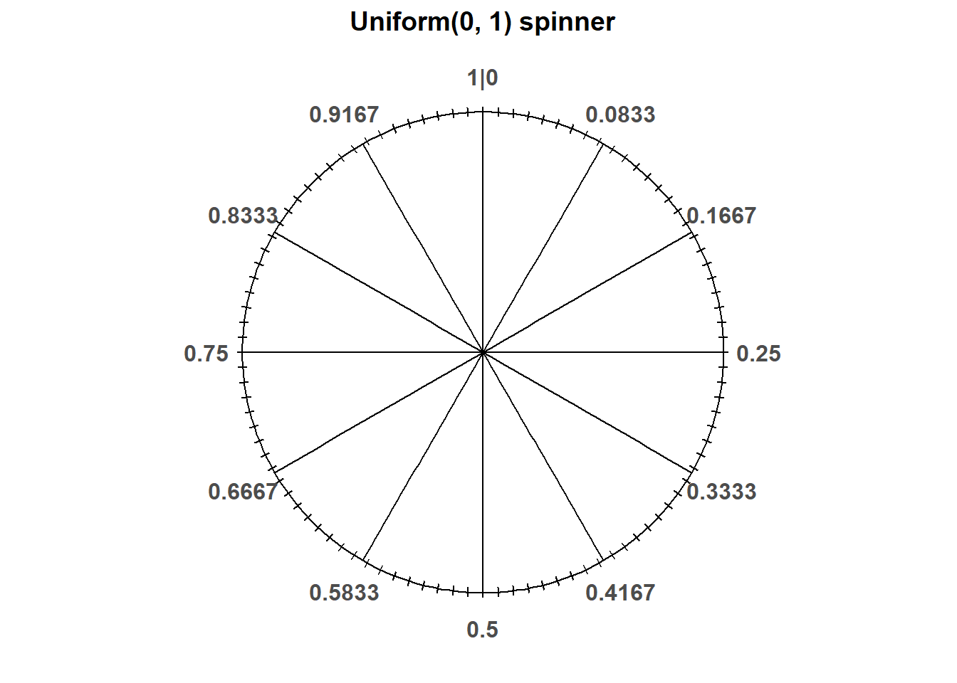
By suitably relabeling the axes on the Uniform(0, 1) spinner, we could have constructed the spinners for any of the other examples.
For example, to obtain the discrete spinner in the middle of Figure 2.6, corresponding to a weighted four-sided die, start with the Uniform(0, 1) spinner and map
- The range (0, 0.1] to 1,
- The range (0.1, 0.3] to 2,
- The range (0.3, 0.6] to 3,
- The range (0.6, 1] to 4
Then the probability that the Uniform(0, 1) spinner lands in the range (0.3, 0.6] is 0.3, so the spinner resulting from this mapping would return a value of 3 with probability 0.3. (The probability of the infinitely precise needle landing on a specific value like 0.3 (that is, \(0.300000000\ldots\)) is 0, so it doesn’t really matter what we do with the endpoints of the intervals.)
For non-uniform values on a continuous scale, we could construct a spinner according to the distribution of interest by rescaling and stretching/shrinking the axis of the Uniform(0, 1) spinner to correspond to intervals of larger/smaller probability. For example, if we want to simulate values according to the Exponential(1) distribution we could start with the Uniform(0, 1) spinner and then transform the axis values \(u \mapsto -\log(1-u)\) to obtain the spinner in Figure 4.13.
In Section 4.3 we started with the transformation \(u\mapsto -\log(1-u)\) of the Uniform(0, 1) spinner and saw what distribution the transformed values followed via simulation (i.e., Exponential(1)). But what about the reverse question: given a particular distribution, how do we find the transformation of Uniform(0, 1) that will generate values according to the specified distribution?
Recall how the spinner in Figure 4.13 was constructed. We started with the Uniform(0, 1) spinner with equally spaced increments, and applied the transformation \(-\log(1-u)\), which “stretched” the intervals corresponding to higher probability and “shrunk” the intervals corresponding to lower probability. The distribution that we ended up with was the Exponential(1) distribution with cdf \(1-e^{-x}, x>0\). Notice now that the transformation \(-\log(1-u)\) corresponds to the quantile function of an Exponential(1) distribution. For example, we want to label the 75th percentile of the Exponential(1) distribution on the axis 75% of the way around the spinner; the quantile function tells us what the 75th percentile is so we know what value to put on the axis.
Example 4.22 provides an example of how to go backwards. Starting from a cdf, we can construct the corresponding spinner by finding the quantile function, essentially the inverse cdf, and applying it to the equally spaced values on the Uniform(0, 1) spinner. The quantile function will stretch/shrink the intervals just right to correspond to the probabilities given by the cdf.
Example 4.23 Recall Example 4.12 where Regina’s arrival time \(X\) (in hours) had pdf \[ f_X(x) = 2x, \qquad 0<x<1. \]
- Find the cdf of \(X\).
- Find the quantile function of \(X\).
- Construct a spinner for simulating values of \(X\) (hours) according to its distribution.
- If we measure \(X\) in minutes, how would the spinner change?
Solution. to Example 4.23
Show/hide solution
- Integrate the pdf: \(F_X(x) = x^2, 0 < x < 1\) (and \(F_X(x) = 0\) if \(x<0\) and \(F_X(x) = 1\) if \(x>1\)).
- Invert the cdf: \(p = F(x) = x^2\) implies \(x = \sqrt{p}\), so \(Q(p) = \sqrt{p}\) for \(0<p<1\).
- Transform the axis of the Uniform(0, 1) spinner using \(u\mapsto \sqrt{u}\). For example, the 25th percentile is \(Q(0.25) = \sqrt{0.25} = 0.5\) (hours), the 50th percentile is \(Q(0.5) = \sqrt{0.5} = 0.707\) (hours), and the 75th percentile is \(Q(0.75) = \sqrt{0.75} = 0.866\) (hours). Notice that the transformation \(u\mapsto \sqrt{u}\) stretches out intervals near 1, the intervals with higher density, and shrinks intervals near 0, the intervals with lower density.
- Changing from hours to minutes is a linear rescaling, so it will just relabel the axis without any differential stretching/shrinking. Simply multiple all the values on the axis by 60.
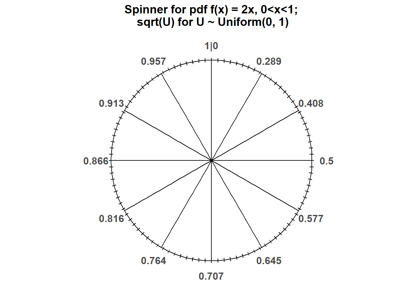
Figure 4.21: Spinner for \(X\) in Example 4.23. The axis is transformed according to the quantile function \(Q(p) = \sqrt{p}\).
These examples illustrate “universality of the uniform”. Basically, we can always start with a spinner that lands uniformly in (0, 1) and suitably stretch/scale the axis around the spinner to construct a spinner corresponding to any distribution of interest. The Uniform(0, 1) spinner returns a value in (0, 1); we obtain the value of the corresponding percentile from the quantile function.
Universality of the Uniform (or “one spinner to rule them all”). Let \(F\) be a cdf and \(Q\) its corresponding quantile function. Let \(U\) have a Uniform(0, 1) distribution and define the random variable \(X=Q(U)\). Then113 the cdf of \(X\) is \(F\).
In the above, \(U\) represents the result of the spin on the [0, 1] scale, and \(Q(U)\) is the corresponding value on the stretched/shrunk scale. \(U\) also represents the area inside the spinner, while \(Q(U)\) represents the value on the circular axis with that area to the left of it.
Universality of the uniform might look complicated but all it basically says is that you can construct a spinner by putting the 25th percentile 25% of the way around, the 75th percentile 75% of the way around, etc.
Actually, universality of the uniform says we don’t have to create a new spinner. We can just spin the Uniform(0, 1) spinner and transform each resulting value by plugging it into the quantile function.
Here is such a simulation for Example 4.23. Notice that the histogram of simulated \(X\) values has the desired shape of the pdf.
U = RV(Uniform(0, 1))

X = sqrt(U)X.sim(10000).plot()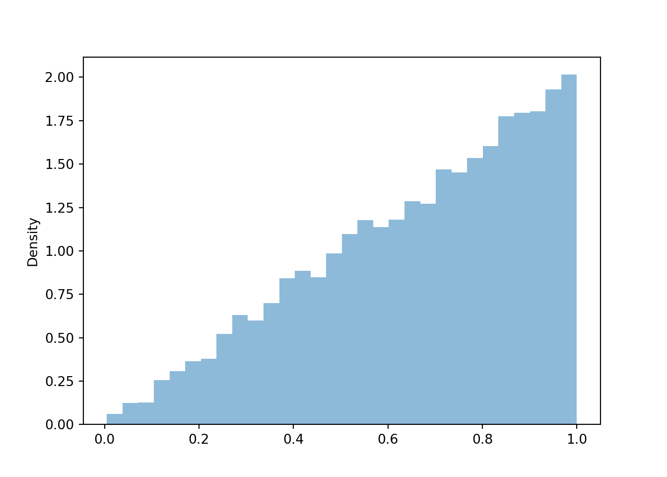
The only examples we have seen where a single spin of a rescaled Uniform(0, 1) distribution would not work were Bivariate Normal distributions, where we described a “globe” for simulating values. However, Example 2.63 introduced a method for simulating from a Bivariate Normal distribution using two spins of the standard Normal spinner. Since the standard Normal spinner can be derived from a Uniform(0, 1) spinner, we can in principle use a Uniform(0, 1) distribution to simulate values from a Bivariate Normal distribution, but we need to spin it twice to generate a single pair.
If the cdf is a continuous function, then the quantile function is the inverse cdf. But the inverse of a cdf might not exist, if the cdf has jumps or flat spots. In particular, the inverse cdf does not exist for discrete random variables. So in general, the quantile function corresponding to cdf \(F\) is defined as \(Q(p) = \inf\{u:F(u)\ge p\}\).↩︎
We’ll only prove the result assuming \(F\) is a continuous, strictly increasing function, so that the quantile function is just the inverse of \(F\), \(Q(p) = F^{-1}(p)\). First note that \(\{F^{-1}(U)\le x\} = \{U\le F(x)\}\); to see why draw a picture like Figure ???. Then \[ \textrm{P}(X \le x) = \textrm{P}(Q(U) \le x) = \textrm{P}(F^{-1}(U)\le x) = \textrm{P}(U\le F(x)) = F(x) \] The last step follows since \(F(x)\) is just a number in [0, 1] and \(\textrm{P}(U\le u) = u\) for \(0\le u\le 1\) since \(U\) has a Uniform(0, 1) distribution.↩︎