4.2 Discrete random variables: Probability mass functions
Discrete random variables take at most countably many possible values (e.g. \(0, 1, 2, \ldots\)). They are often, but not always, counting variables (e.g., \(X\) is the number of Heads in 10 coin flips). We have seen in several examples that the distribution of a discrete random variable can be specified via a table listing the possible values of \(x\) and the corresponding probability \(\textrm{P}(X=x)\). Always be sure to specify the possible values of \(X\).
In some cases, the distribution has a “formulaic” shape and \(\textrm{P}(X=x)\) can be written explicitly as a function of \(x\). For example, let \(X\) be the sum of two rolls of a fair four-sided die. The distribution of \(X\) is displayed below. The probabilities of the possible \(x\) values follow a clear triangular pattern as a function of \(x\).
| x | P(X=x) |
|---|---|
| 2 | 0.0625 |
| 3 | 0.1250 |
| 4 | 0.1875 |
| 5 | 0.2500 |
| 6 | 0.1875 |
| 7 | 0.1250 |
| 8 | 0.0625 |
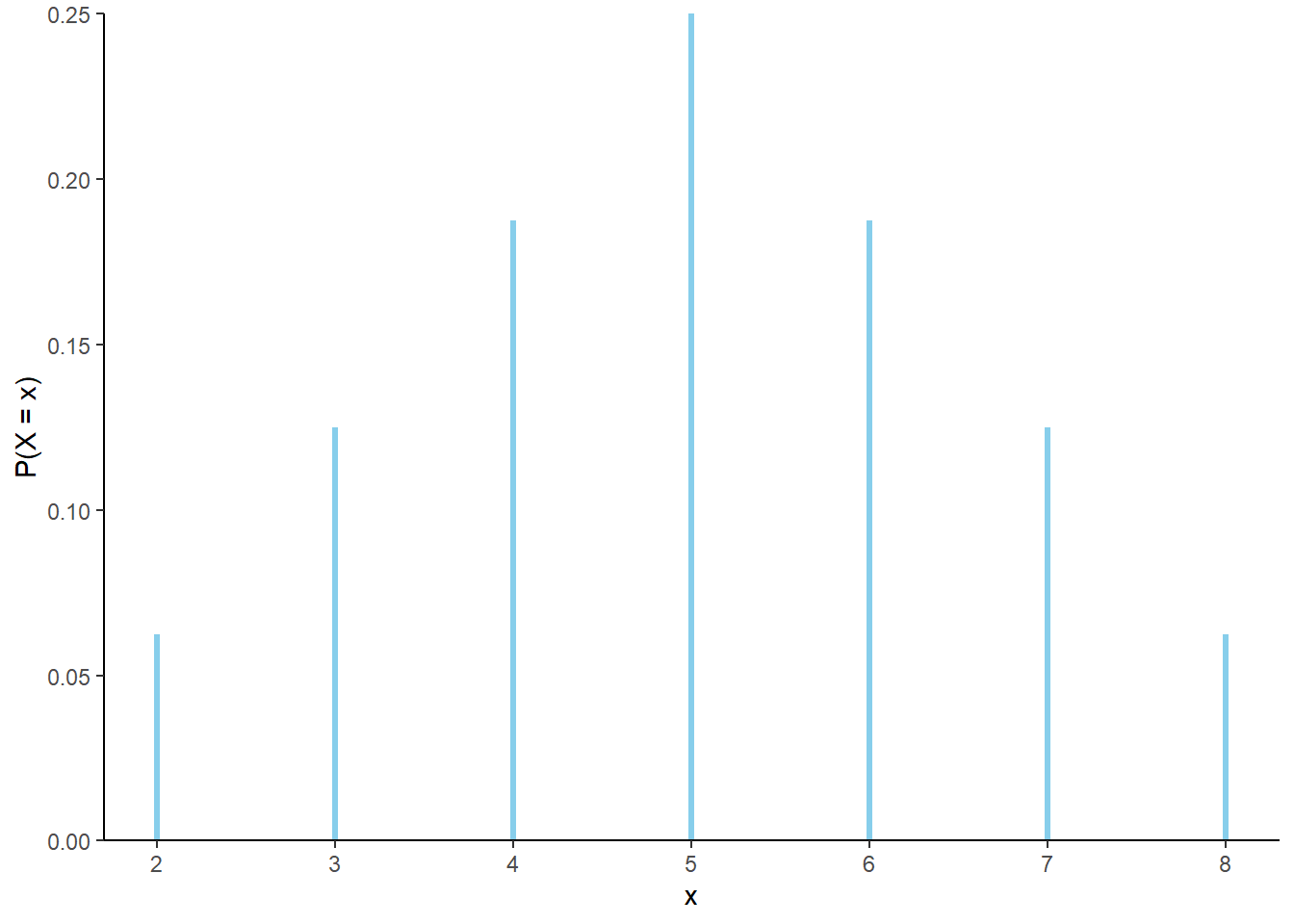
Figure 4.1: The marginal distribution of \(X\), the sum of two rolls of a fair four-sided die.
For each possible value \(x\) of the random variable \(X\), \(\textrm{P}(X=x)\) can be obtained from the following formula
\[ p(x) = \begin{cases} \frac{4-|x-5|}{16}, & x = 2, 3, 4, 5, 6,7, 8,\\ 0, & \text{otherwise.} \end{cases} \]
That is, \(\textrm{P}(X = x) = p(x)\) for all \(x\). For example, \(\textrm{P}(X = 2) = 1/16 = p(2)\); \(\textrm{P}(X=5)=4/16=p(5)\); \(\textrm{P}(X=7.5)=0=p(7.5)\). To specify the distribution of \(X\) we could provide Table 4.1, or we could just provide the function \(p(x)\) above. Notice that part of the specification of \(p(x)\) involves the possible values of \(x\); \(p(x)\) is only nonzero for \(x=2,3, \ldots, 8\). Think of \(p(x)\) as a compact way of representing Table 4.1. The function \(p(x)\) is called the probability mass function of the discrete random variable \(X\).
Definition 4.1 The probability mass function (pmf) (a.k.a., density (pdf)101) of a discrete RV \(X\), defined on a probability space with probability measure \(\textrm{P}\), is a function \(p_X:\mathbb{R}\mapsto[0,1]\) which specifies each possible value of the RV and the probability that the RV takes that particular value: \(p_X(x)=\textrm{P}(X=x)\) for each possible value of \(x\).
The axioms of probability imply that a valid pmf must satisfy \[\begin{align*} p_X(x) & \ge 0 \quad \text{for all $x$}\\ p_X(x) & >0 \quad \text{for at most countably many $x$ (the possible values, i.e., support)}\\ \sum_x p_X(x) & = 1 \end{align*}\]
The countable set of possible values of a discrete random variable \(X\), \(\{x: \textrm{P}(X=x)>0\}\), is called its support.
The pmf of a discrete random variable provides the probability of “equal to” events: \(\textrm{P}(X = x)\). Probabilities for other general events, e.g., \(\textrm{P}(X \le x)\) can be obtained by summing the pmf over the range of values of interest.
We have seen that a distribution of a discrete random variable can be represented in a table, with a corresponding spinner. Think of a pmf as providing a compact formula for constructing the table/spinner.
Example 4.4 Let \(Y\) be the larger of two rolls of a fair four-sided die. Find the probability mass function of \(Y\).
Solution. to Example 4.4
Show/hide solution
See Table 4.2 and Figure 4.2 below. As a function of \(y=1, 2, 3, 4\), \(\textrm{P}(Y=y)\) is linear with slope 2/16 passing through the point (1, 1/16). The pmf of \(Y\) is
\[ p_Y(y) = \begin{cases} \frac{2y-1}{16}, & y = 1, 2, 3, 4, \\ 0, & \text{otherwise.} \end{cases} \]
For any \(y\), \(\textrm{P}(Y=y) = p_Y(y)\). For example, \(\textrm{P}(Y=2) = 3/16 = p_Y(2)\) and \(\textrm{P}(Y = 3.3) = 0 = p_Y(3.3)\).
| y | P(Y=y) |
|---|---|
| 1 | 0.0625 |
| 2 | 0.1875 |
| 3 | 0.3125 |
| 4 | 0.4375 |
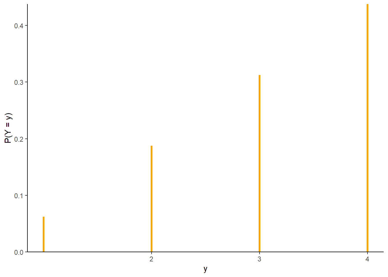
Figure 4.2: The marginal distribution of \(Y\), the larger (or common value if a tie) of two rolls of a fair four-sided die.
Example 4.5 Donny Dont provides two answers to Example 4.4. Are his answers correct? If not, why not?
- \(p_Y(y) = \frac{2y-1}{16}\)
- \(p_Y(x) = \frac{2x-1}{16},\; x = 1, 2, 3, 4\), and \(p_Y(x)= 0\) otherwise.
Solution. to Example 4.5
Show/hide solution
- Donny’s solution is incomplete; he forgot to specify the possible values. It’s possible that someone who sees Donny’s expression would think that \(p_Y(2.5)=4/16\). You don’t necessarily always need to write “0 otherwise”, but do always provide the possible values.
- Donny’s answer is actually correct, though maybe a little confusing. The important place to put a \(Y\) is the subscript of \(p\): \(p_Y\) identifies this function as the pmf of the random variable \(Y\), as opposed to any other random variable that might be of interest. The argument of \(p_Y\) is just a dummy variable that defines the function. As an analogy, \(g(u)=u^2\) is the same function as \(g(x)=x^2\); it doesn’t matter which symbol defines the argument. It is convenient to represent the argument of the pmf of \(Y\) as \(y\), and the argument of the pmf of \(X\) as \(x\), but this is not necessary. Donny’s answer does provide a way of constructing Table 2.12.
When there are multiple discrete random variables of interest, we usually identify their marginal pmfs with subscripts: \(p_X, p_Y, p_Z\), etc.
4.2.1 Benford’s law
We often specify the distribution of a random variable directly by providing its pmf. Certain common distributions have special names.
Example 4.6 Randomly select a county in the U.S. Let \(X\) be the leading digit in the county’s population. For example, if the county’s population is 10,040,000 (Los Angeles County) then \(X=1\); if 3,170,000 (Orange County) then \(X=3\); if 283,000 (SLO County) then \(X=2\); if 30,600 (Lassen County) then \(X=3\). The possible values of \(X\) are \(1, 2, \ldots, 9\). You might think that \(X\) is equally likely to be any of its possible values. However, a more appropriate model102 is to assume that \(X\) has pmf \[ p_X(x) = \begin{cases} \log_{10}(1+\frac{1}{x}), & x = 1, 2, \ldots, 9,\\ 0, & \text{otherwise} \end{cases} \] This distribution is known as Benford’s law.
- Construct a table specifying the distribution of \(X\), and the corresponding spinner.
- Find \(\textrm{P}(X \ge 3)\)
Solution. to Example 4.6
- Table 4.3 and the spinner in Figure 4.3 below specify the distribution of \(X\).
- We can add the corresponding values from the pmf. \(\textrm{P}(X \ge 3) = 1 - \textrm{P}(X <3) = 1 - (0.301 + 0.176) = 0.523\).
| x | p(x) |
|---|---|
| 1 | 0.301 |
| 2 | 0.176 |
| 3 | 0.125 |
| 4 | 0.097 |
| 5 | 0.079 |
| 6 | 0.067 |
| 7 | 0.058 |
| 8 | 0.051 |
| 9 | 0.046 |
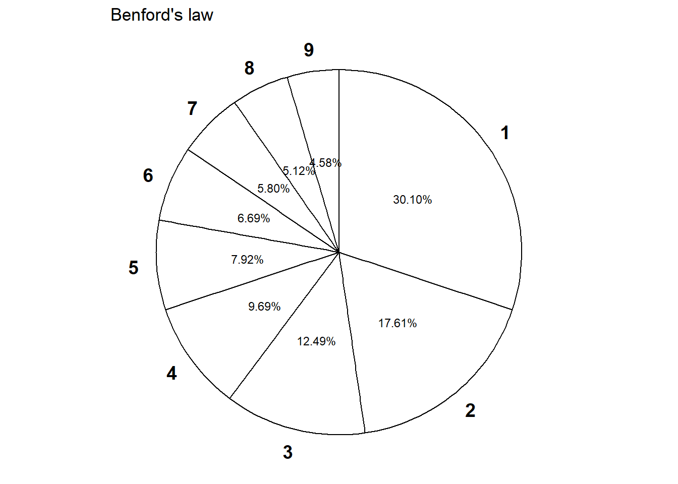
Figure 4.3: Spinner corresponding to Benford’s law.
4.2.2 Poisson distributions
Poisson distributions are often used to model random variables that count “relatively rare events”.
Example 4.7 Let \(X\) be the number of home runs hit (in total by both teams) in a randomly selected Major League Baseball game. Technically, there is no fixed upper bound on what \(X\) can be, so mathematically it is convenient to consider \(0, 1, 2, \ldots\) as the possible values of \(X\). Assume that the pmf of \(X\) is
\[ p_X(x) = \begin{cases} e^{-2.3} \frac{2.3^x}{x!}, & x = 0, 1, 2, \ldots\\ 0, & \text{otherwise.} \end{cases} \]
This is known as the Poisson(2.3) distribution.
- Verify that \(p_X\) is a valid pmf.
- Compute \(\textrm{P}(X = 3)\), and interpret the value as a long run relative frequency.
- Construct a table and spinner corresponding to the distribution of \(X\).
- Find \(\textrm{P}(X \le 13)\), and interpret the value as a long run relative frequency. (The most home runs ever hit in a baseball game is 13.)
- Find and interpret the ratio of \(\textrm{P}(X = 5)\) to \(\textrm{P}(X = 3)\). Does the value \(e^{-2.3}\) affect this ratio?
- Use simulation to find the long run average value of \(X\), and interpret this value.
- Use simulation to find the variance and standard deviation of \(X\).
Solution. to Example 4.7
Show/hide solution
- We need to verify that the probabilities in the pmf sum to 1. We can construct the corresponding table and just make sure the values sum to 1. Technically, any value \(0, 1, 2, \ldots\) is possible, but the probabilities will get closer and closer to 0 as \(x\) gets larger. So we can cut our table off at some reasonable upper bound for \(X\), where the sum of the values in the table is close enough to 1 for practical purposes. If we wanted to sum over all possible values of \(X\), we need to use the Taylor series expansion of \(e^u\). \[ \sum_{x=0}^\infty e^{-2.3} \frac{2.3^x}{x!} = e^{-2.3} \sum_{x=0}^\infty \frac{2.3^x}{x!} = e^{-2.3}e^{2.3} = 1 \] The constant \(e^{-2.3}\approx0.100\) simply ensures that the probabilities that follow the shape determined by \(2.3^x/ x!\) sum to 1.
- Just plug \(x=3\) into the pmf: \(\textrm{P}(X=3)=p_X(3)=e^{-2.3}2.3^3/3! = 0.203\). In the long run, 20.3% of baseball games have 3 home runs.
- See the table and Figure 4.4 below. Plug each value of \(x\) into the pmf. For example, \(\textrm{P}(X = 5) =p_X(5)=e^{-2.3}2.3^5/5! = 0.054\).
- Just sum the values of the pmf corresponding to the values \(x = 0, 1, \ldots, 13\): \(\textrm{P}(X \le 13) = \sum_{x=0}^{13} p_X(x)=0.9999998\). There isn’t any shorter way to do it. In the long run, almost all MLB games have at most 13 home runs. Even though the pmf assigns nonzero probability to all values 0, 1, 2, \(\ldots\), the probability that \(X\) takes a value greater than 13 is extremely small.
- The ratio is \[ \frac{\textrm{P}(X=3)}{\textrm{P}(X=5)} = \frac{p_X(3)}{p_X(5)} = \frac{e^{-2.3}2.3^3/3!}{e^{-2.3}2.3^5/5!} = \frac{2.3^3/3!}{2.3^5/5!} = 3.78 \] Games with 3 home runs occur about 3.8 times more frequently than games with 5 home runs. The constant \(e^{-2.3}\) does not affect this ratio; see below for further discussion.
- The simulation results below suggest that the long run average value of \(X\) is equal to the parameter 2.3. Over many baseball games there are a total of 2.3 home runs per game on average.
- The simulation results also suggest that variance of \(X\) is equal to 2.3, and the standard deviation of \(X\) is equal to \(\sqrt{2.3}\approx 1.52\).
| \(x\) | \(p(x)\) | Value |
|---|---|---|
| 0 | \(e^{-2.3}\frac{2.3^0}{0!}\) | 0.100259 |
| 1 | \(e^{-2.3}\frac{2.3^1}{1!}\) | 0.230595 |
| 2 | \(e^{-2.3}\frac{2.3^2}{2!}\) | 0.265185 |
| 3 | \(e^{-2.3}\frac{2.3^3}{3!}\) | 0.203308 |
| 4 | \(e^{-2.3}\frac{2.3^4}{4!}\) | 0.116902 |
| 5 | \(e^{-2.3}\frac{2.3^5}{5!}\) | 0.053775 |
| 6 | \(e^{-2.3}\frac{2.3^6}{6!}\) | 0.020614 |
| 7 | \(e^{-2.3}\frac{2.3^7}{7!}\) | 0.006773 |
| 8 | \(e^{-2.3}\frac{2.3^8}{8!}\) | 0.001947 |
| 9 | \(e^{-2.3}\frac{2.3^9}{9!}\) | 0.000498 |
| 10 | \(e^{-2.3}\frac{2.3^{10}}{10!}\) | 0.000114 |
| 11 | \(e^{-2.3}\frac{2.3^{11}}{11!}\) | 0.000024 |
| 12 | \(e^{-2.3}\frac{2.3^{12}}{12!}\) | 0.000005 |
| 13 | \(e^{-2.3}\frac{2.3^{13}}{13!}\) | 0.000001 |
| 14 | \(e^{-2.3}\frac{2.3^{14}}{14!}\) | 0.000000 |
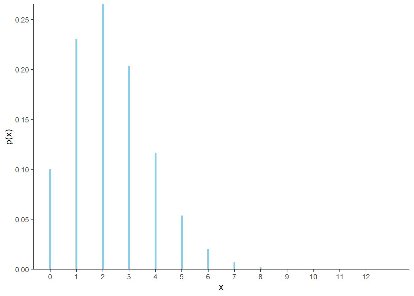
Figure 4.4: Impulse plot representing the Poisson(2.3) probability mass function.
Figure 4.5 displays a spinner corresponding to the Poisson(2.3) distribution. To simplify the display we have lumped all values \(6, 7, \ldots\) into one “6+” category.
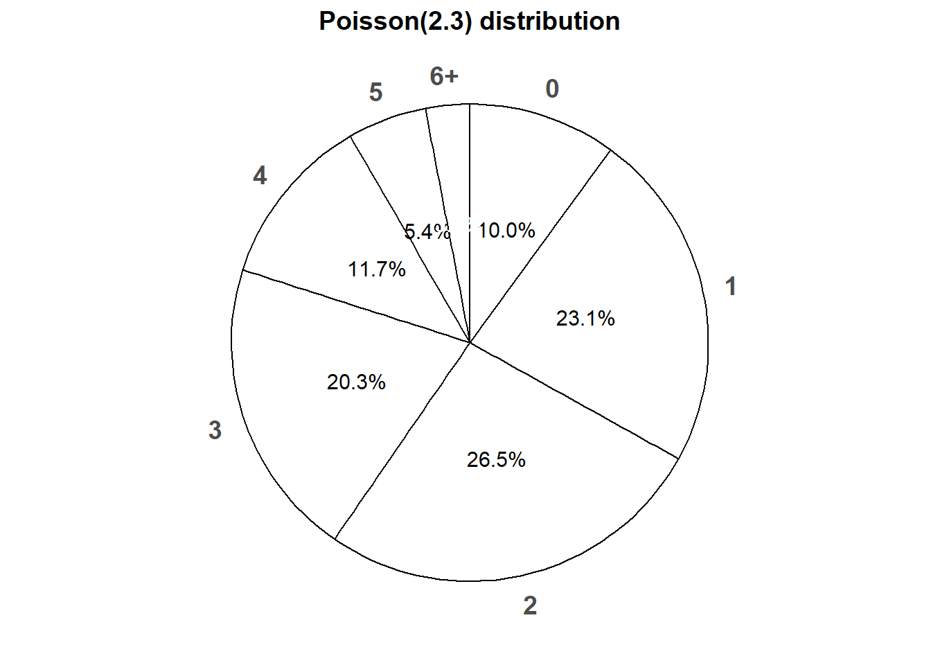
Figure 4.5: Spinner corresponding to the Poisson(2.3) distribution.
The constant \(e^{-2.3}\) doesn’t affect the shape of the probability mass function. Rather, the constant \(e^{-2.3}\) is what ensures that the probabilities sum to 1. We could have written the pmf as
\[ p_X(x) \propto \begin{cases} \frac{2.3^x}{x!}, & x = 0, 1, 2, \ldots\\ 0, & \text{otherwise.} \end{cases} \]
The symbol \(\propto\) means “is proportional to”. This specification is enough to determine the shape of the distribution and relative likelihoods. For example, the above is enough to determine that the probability that \(X\) takes the value 3 is 3.78 times greater than the probability that \(X\) takes the value 5. Once we have the shape of the distribution, we can “renormalize” by multiplying all values by a constant, in this case \(e^{-2.3}\), so that the values sum to 1. We saw a similar idea in Example 1.5. The constant is whatever it needs to be so that the values sum to 1; what’s important is the relative shape. The “is proportional to” specification defines the shape of the plot; the constant just rescales the values on the probability axis.
Why might we assume this particular Poisson(2.3) distribution for the number of home runs per game? We’ll discuss this point in more detail later. For now we’ll just present Figure 4.6 which displays the actual distribution of home runs over the 2431 games in the 2018 MLB season. The spikes represent the observed relative frequencies; the connecting dots represent the theoretical Poisson(2.3) pmf. We can see that the Poisson(2.3) distribution models the data reasonably well.
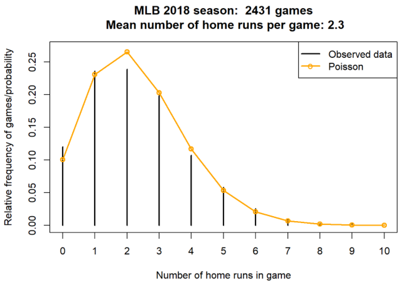
Figure 4.6: Data on home runs per game in the 2018 MLB season, compared with the Poisson(2.3) distribution.
A general Poisson distribution is defined by a single parameter \(\mu>0\). (In the home run example, \(\mu=2.3\).)
Definition 4.2 A discrete random variable \(X\) has a Poisson distribution with parameter103 \(\mu>0\) if its probability mass function \(p_X\) satisfies \[\begin{align*} p_X(x) & \propto \frac{\mu^x}{x!}, \;\qquad x=0,1,2,\ldots\\ & = \frac{e^{-\mu}\mu^x}{x!}, \quad x=0,1,2,\ldots \end{align*}\] The function \(\mu^x / x!\) defines the shape of the pmf. The constant \(e^{-\mu}\) ensures that the probabilities sum to 1.
If \(X\) has a Poisson(\(\mu\)) distribution then \[\begin{align*} \text{Long run average value of $X$} & = \mu\\ \text{Variance of $X$} & = \mu\\ \text{SD of $X$} & = \sqrt{\mu} \end{align*}\]
There is not one “Poisson distribution” but rather a family of Poisson distributions. Each Poisson distribution follows the general pattern specified by the Poisson pmf, with the particular shape determined by the parameter \(\mu\). While the possible values of a variable that follows a Poisson distribution are nonnegative integers, the parameter \(\mu\) can be any positive value.
Poisson(1).plot()
Poisson(2.3).plot()
Poisson(2.5).plot()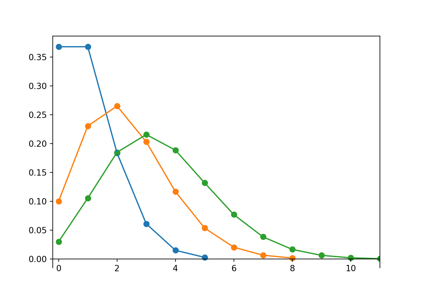
We will see more properties and uses of Poisson distributions later.
In Symbulate we can define a random variable with a Poisson(2.3) distribution and simulate values.
X =  RV(Poisson(2.3))

x = X.sim(10000)
x| Index | Result |
|---|---|
| 0 | 1 |
| 1 | 2 |
| 2 | 2 |
| 3 | 2 |
| 4 | 2 |
| 5 | 2 |
| 6 | 4 |
| 7 | 1 |
| 8 | 1 |
| ... | ... |
| 9999 | 5 |
The spikes in the plot below correspond to simulated relative frequencies.
The connecting dots displayed by Poisson(2.3).plot() are determined by the theoretical Poisson(2.3) pmf.
x.plot() # plot the simulated values and their relative frequencies

Poisson(2.3).plot() # plot the theoretical Poisson(2.3) pmf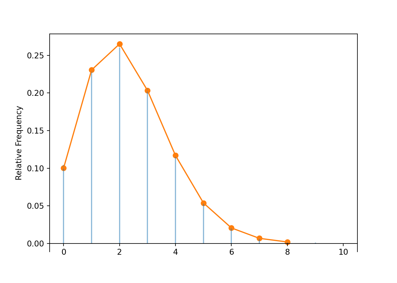
The approximate long run average value and variance are both about equal to the parameter 2.3.
x.mean(), x.var(), x.sd()## (2.2897, 2.3227739099999996, 1.524064929719203)The Symbulate pmf method can be used to compute the pmf for named distributions.
The following compares the simulated relative frequency of \(\{X = 3\}\) to the theoretical probability \(p_X(3)\).
x.count_eq(3) / x.count(), Poisson(2.3).pmf(3)## (0.206, 0.20330822526255884)You can evaluate the pmf at multiple values.
xs = list(range(5)) # the values 0, 1, ..., 4

Poisson(2.3).pmf(xs)
## array([0.10025884, 0.23059534, 0.26518464, 0.20330823, 0.11690223])Below we use the Python package tabulate to construct a somewhat nicer table.
Don’t get this tabulate confused with .tabulate() in Symbulate.
xs = list(range(14)) # the values 0, 1, ..., 13

from tabulate import tabulate

print(tabulate({'x': xs,
                'p_X(x)': [Poisson(2.3).pmf(u) for u in xs]},
               headers = 'keys', floatfmt=".6f"))
## x p_X(x)
## --- --------
## 0 0.100259
## 1 0.230595
## 2 0.265185
## 3 0.203308
## 4 0.116902
## 5 0.053775
## 6 0.020614
## 7 0.006773
## 8 0.001947
## 9 0.000498
## 10 0.000114
## 11 0.000024
## 12 0.000005
## 13 0.000001We can obtain \(\textrm{P}(X \le 13)\) by summing the corresponding probabilities from the pmf.
We can also find \(\textrm{P}(X \le 13)\) by evaluating the cdf at 13.
(We will see more about cumulative distribution functions (cdfs) soon.)
Poisson(2.3).pmf(xs).sum(), Poisson(2.3).cdf(13)## (0.9999998428405235, 0.9999998428405236)4.2.3 Binomial distributions
In some cases, a pmf of a discrete random variable can be derived from the assumptions about the underyling random phenomenon.
Example 4.8 Capture-recapture sampling is a technique often used to estimate the size of a population. Suppose you want to estimate \(N\), the number of monarch butterflies in Pismo Beach. (Assume that \(N\) is a fixed but unknown number; the population size doesn’t change over time.) You first capture a sample of \(N_1\) butterflies, selected randomly, and tag them and release them. At a later date, you then capture a second sample of \(n\) butterflies, selected randomly104 with replacement. Let \(X\) be the number of butterflies in the second sample that have tags (because they were also caught in the first sample). (Assume that the tagging has no effect on behavior, so that selection in the first sample is independent of selection in the second sample.)
In practice, \(N\) is unknown and the point of capture-recapture sampling is to estimate \(N\). But let’s start with a simpler, but unrealistic, example where there are \(N=52\) butterflies, \(N_1 = 13\) are tagged and \(N_0=52-13 = 39\) are not, and \(n=5\) is the size of the second sample.
- Explain why it is reasonable to assume that the results of the five individual selections are independent.
- Compute and interpret \(\textrm{P}(X=0)\).
- Compute the probability that the first butterfly selected is tagged but the others are not.
- Compute the probability that the last butterfly selected is tagged but the others are not.
- Compute and interpret \(\textrm{P}(X=1)\).
- Compute and interpret \(\textrm{P}(X=2)\).
- Find the pmf of \(X\).
- Construct a table, plot, and spinner representing the distribution of \(X\).
- Make an educated guess for the long run average value of \(X\).
- How do the results depend on \(N_1\) and \(N_0\)?
Solution. to Example 4.8
Show/hide solution
- Since the selections are made with replacement, at the time of each selection there are 52 butterflies of which 13 are tagged, regardless of the results of previous selections. That is, for each selection the conditional probability that a butterfly is tagged is 13/52 regardless of the results of other selections.
- Let S (for “success”) represent that a selected butterfly is tagged, and F (for “failure”) represent that it’s not tagged. None of the 5 butterflies are tagged if the selected sequence is FFFFF. Since the selections are independent \[ \textrm{P}(X = 0) = \left(\frac{39}{52}\right)\left(\frac{39}{52}\right)\left(\frac{39}{52}\right)\left(\frac{39}{52}\right)\left(\frac{39}{52}\right) = \left(\frac{39}{52}\right)^5 = 0.237 \] Repeating the process in the long run means drawing many samples of size 5: 23.7% of samples of size 5 will have 0 tagged butterflies.
- Since the selections are independent, the probability of the outcome SFFFF is \[ \left(\frac{13}{52}\right)\left(\frac{39}{52}\right)\left(\frac{39}{52}\right)\left(\frac{39}{52}\right)\left(\frac{39}{52}\right) = \left(\frac{13}{52}\right)\left(\frac{39}{52}\right)^4 = 0.079 \]
- The probability of the outcome FFFFS is the same as in the previous part \[ \left(\frac{13}{52}\right)\left(\frac{39}{52}\right)^4 = 0.079 \]
- Each of the particular outcomes with 1 tagged butterfly has probability \(\left(\frac{13}{52}\right)\left(\frac{39}{52}\right)^4=0.079\). So we need to count how many outcomes result in 1 tagged butterfly. Since there are 5 “spots” where the 1 tagged butterfly can be, there are \(\binom{5}{1}=5\) such sequences (SFFFF, FSFFF, FFSFF, FFFSF, FFFFS) \[ \textrm{P}(X = 1) = \binom{5}{1}\left(\frac{13}{52}\right)\left(\frac{39}{52}\right)^4 = 5(0.079) = 0.3955 \] 39.6% of samples of size 5 will have exactly 1 tagged butterfly.
- Each of the particular outcomes with 2 tagged butterflies (like SSFFF) has probability \(\left(\frac{13}{52}\right)^2\left(\frac{39}{52}\right)^3=0.02637\). Since there are 5 “spots” where the 2 tagged butterflies can be, there are \(\binom{5}{2}=10\) such sequences.
\[ \textrm{P}(X = 2) = \binom{5}{2}\left(\frac{13}{52}\right)^2\left(\frac{39}{52}\right)^3 = 10(0.02637) = 0.2637 \] 26.4% of samples of size 5 will have exactly 2 tagged butterflies. - Similar to the previous part. Any particular outcome with \(x\) successes has \(5-x\) failures. The probability of any particular outcomes with exactly \(x\) successes (and \(5-x\) failures) is \((13/52)^x(39/52)^{5-x}\). There are \(\binom{5}{x}\) outcomes that result in exactly \(x\) successes, so the total probability of \(x\) successes is \[ p_X(x) = \binom{5}{x}\left(\frac{13}{52}\right)^x\left(\frac{39}{52}\right)^{5-x}, \qquad x = 0, 1, 2, 3, 4, 5 \]
- See below. Plug each possible value into the pmf from the previous part.
- If 1/4 of the butterflies in the population are tagged, we would also expect 1/4 of the butterflies in a randomly selected sample to be tagged. We would expect the long run average value to be \(5(13/52) = 1.25\).
- The results only depend on \(N_1\) and \(N_0\) through the ratio \(13/52 = N_1/(N_0+N_1)\). That is, when the selections are made with replacement, only the population proportion is needed. If we had only been told that 25% of the butterflies were tagged, instead of 13 out of 52, we still could have solved the problem and nothing would change.
The distribution of \(X\) in the previous problem is called the Binomial(5, 0.25) distribution. The parameter 5 is the size of the sample, and the parameter 0.25 is the proportion of successes in the population.
| \(x\) | \(p(x)\) | Value |
|---|---|---|
| 0 | \(\binom{5}{0}0.25^0(1-0.25)^{5-0}\) | 0.237305 |
| 1 | \(\binom{5}{1}0.25^1(1-0.25)^{5-1}\) | 0.395508 |
| 2 | \(\binom{5}{2}0.25^2(1-0.25)^{5-2}\) | 0.263672 |
| 3 | \(\binom{5}{3}0.25^3(1-0.25)^{5-3}\) | 0.087891 |
| 4 | \(\binom{5}{4}0.25^4(1-0.25)^{5-4}\) | 0.014648 |
| 5 | \(\binom{5}{5}0.25^5(1-0.25)^{5-5}\) | 0.000977 |
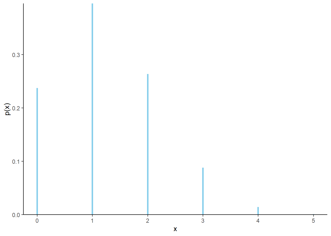
Figure 4.7: Impulse plot representing the Binomial(5, 0.25) probability mass function.
Figure 4.8 displays a spinner corresponding to the Binomial(5, 0.25) distribution. To simplify the display we have lumped 4 and 5 into one “4+” category.
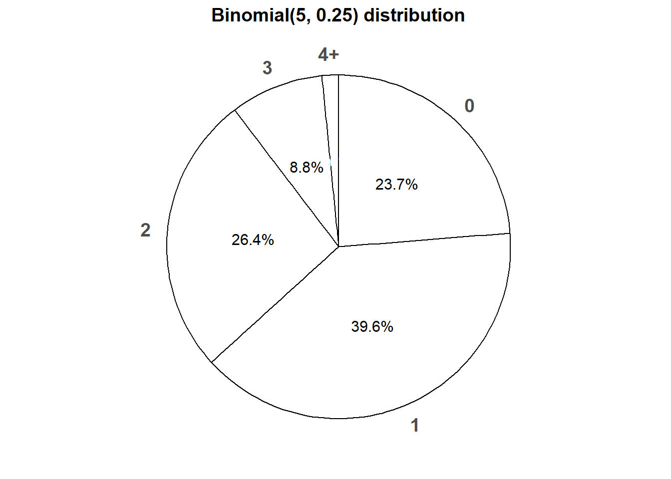
Figure 4.8: Spinner corresponding to the Binomial(5, 0.25) distribution.
Definition 4.3 A discrete random variable \(X\) has a Binomial distribution with parameters \(n\), a nonnegative integer, and \(p\in[0, 1]\) if its probability mass function is \[\begin{align*} p_{X}(x) & = \binom{n}{x} p^x (1-p)^{n-x}, & x=0, 1, 2, \ldots, n \end{align*}\] If \(X\) has a Binomial(\(n\), \(p\)) distribution then \[\begin{align*} \text{Long run average value of $X$} & = np\\ \text{Variance of $X$} & = np(1-p)\\ \text{SD of $X$} & = \sqrt{np(1-p)} \end{align*}\]
Imagine a box containing tickets with \(p\) representing the proportion of tickets in the box labeled 1 (“success”); the rest are labeled 0 (“failure”). Randomly select \(n\) tickets from the box with replacement and let \(X\) be the number of tickets in the sample that are labeled 1. Then \(X\) has a Binomial(\(n\), \(p\)) distribution. Since the tickets are labeled 1 and 0, the random variable \(X\) which counts the number of successes is equal to the sum of the 1/0 values on the tickets. If the selections are made with replacement, the draws are independent, so it is enough to just specify the population proportion \(p\) without knowing the population size \(N\).
The situation in the previous paragraph and the butterfly example involves a sequence of Bernoulli trials.
- There are only two possible outcomes, “success” (1) and “failure” (0), on each trial.
- The unconditional/marginal probability of success is the same on every trial, and equal to \(p\)
- The trials are independent.
If \(X\) counts the number of successes in a fixed number, \(n\), of Bernoulli(\(p\)) trials then \(X\) has a Binomial(\(n, p\)) distribution.
Careful: Don’t confuse the number \(p\), the probability of success on any single trial, with the probability mass function \(p_X(\cdot)\) which takes as an input a number \(x\) and returns as an output the probability of \(x\) successes in \(n\) Bernoulli(\(p\)) trials, \(p_X(x)=\textrm{P}(X=x)\).
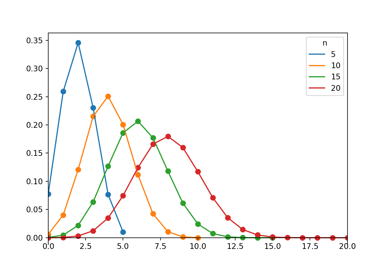
Figure 4.9: Probability mass functions for Binomial(\(n\), 0.4) distributions for \(n = 5, 10, 15, 20\).
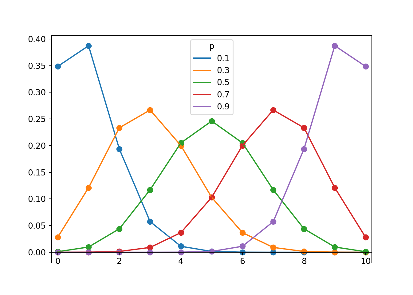
Figure 4.10: Probability mass functions for Binomial(10, \(p\)) distributions for \(p = 0.1, 0.3, 0.5, 0.7, 0.9\).
We will study more properties and uses of Binomial distributions later.
Now we simulate a sample of size 5 with replacement from a box model with 52 tickets, 12 labeled 1 (success) and 39 labeled 0 (failure).
With 1/0 representing S/F, we can also obtain the number of successes with X = RV(P, sum).
P = BoxModel({1: 13, 0: 39}, size = 5, replace = True)

X = RV(P, count_eq(1))

x = X.sim(10000)

x| Index | Result |
|---|---|
| 0 | 1 |
| 1 | 2 |
| 2 | 1 |
| 3 | 0 |
| 4 | 1 |
| 5 | 1 |
| 6 | 0 |
| 7 | 1 |
| 8 | 2 |
| ... | ... |
| 9999 | 3 |
x.plot() # plot the simulated values and their relative frequencies

Binomial(n = 5, p = 13 / 52).plot() # plot the theoretical Binomial(5, 0.25) pmf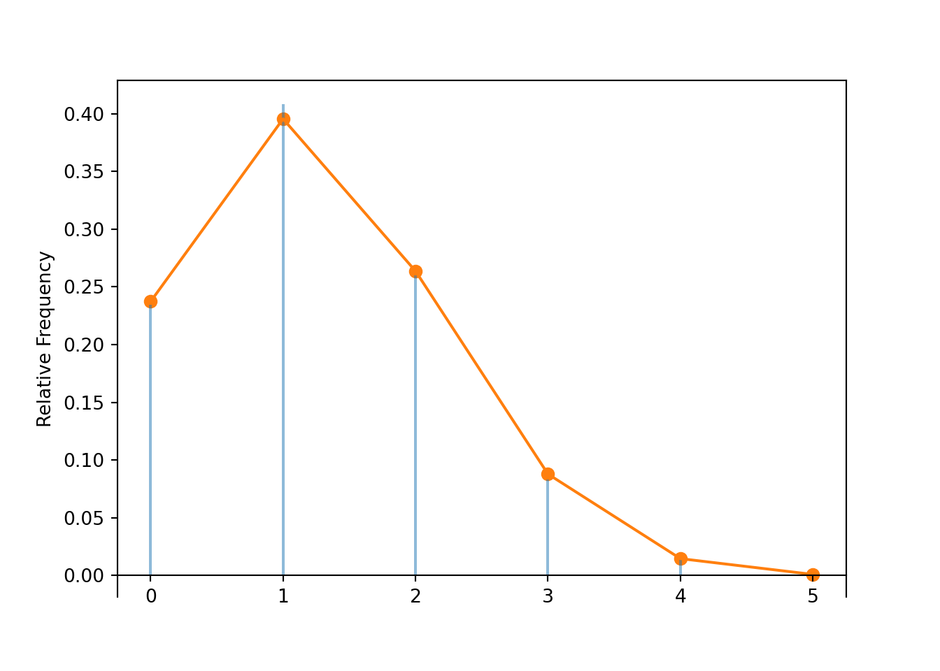
Compare the approximate \(\textrm{P}(X = 2)\) to the theoretical value.
x.count_eq(2) / 10000, Binomial(n = 5, p = 13 / 52).pmf(2)## (0.2598, 0.26367187499999994)Compare the simulated average value of \(X\) to the theoretical long run average value.
x.mean(), Binomial(n = 5, p = 13 / 52).mean()## (1.2345, 1.25)Compare the simulated average value of \(X\) to the theoretical long run average value.
x.var(), Binomial(n = 5, p = 13 / 52).var()## (0.90350975, 0.9375)We use “pmf” for discrete distributions and reserve “pdf” for continuous probability density functions. The terms “pdf” and “density” are sometimes used in both discrete and continuous situations even though the objects the terms represent differ between the two situations (probability versus density). In particular, in R the
dcommands (dbinom,dnorm, etc) are used for both discrete and continuous distributions. In Symbulate, you can use.pmf()for discrete distributions.↩︎In a wide variety of data sets, the leading digit follows Benford’s law. This Shiny app has a few examples. Benford’s law is often used in fraud detection. In particular, if the leading digits in a series of values follows a distribution other than Benford’s law, such as discrete uniform, then there is evidence that the values might have been fudged. Benford’s law has been used recently to test reliability of reported COVID-19 cases and deaths. Here is a nice explanation of why leading digits might follow Benford’s law in data sets that span multiple orders of magnitude↩︎
The parameter for a Poisson distribution is often denoted \(\lambda\). However, we use \(\mu\) to denote the parameter of a Poisson distribution, and reserve \(\lambda\) to denote the rate parameter of a Poisson process (which has mean \(\lambda t\) at time \(t\)).↩︎
We’ll compare to the case of sampling without replacement later.↩︎