5.3 Variance and standard deviation
The values of a random variable vary. The distribution of a random variable describes its pattern of variability. The expected value of a random variable summarizes the distribution in just a single number, the long run average value. But the expected value does not tell us much125 about the degree of variability of the random variable. Do the values of the random variable tend to be close to the expected value, or are they spread out? Variance and standard deviation are numbers that address these questions.
Example 5.11 A roulette wheel has 18 black spaces, 18 red spaces, and 2 green spaces, all the same size and each with a different number on it. Guillermo bets $1 on black. If the wheel lands on black, Guillermo wins his bet back plus an additional $1; otherwise he loses the money he bet. Let \(W\) be Guillermo’s net winnings (net of the initial bet of $1.)
- Find the distribution of \(W\).
- Compute \(\textrm{E}(W)\).
- Interpret \(\textrm{E}(W)\) in context.
- An expected profit for the casino of 5 cents per $1 bet seems small. Explain how casinos can turn such a small profit into billions of dollars.
- In Section 2.10 we introduced variance as the long run average squared distance from the mean. Describe how you could use simulation to approximate the variance of \(W\). What would you expect the simulation results to look like?
- Without doing any further calculations, provide a ballpark estimate of the variance. Explain. What are the measurement units for the variance?
- The random variable \((W-\textrm{E}(W))^2\) represents the squared deviation from the mean. Find the distribution of this random variable and its expected value.
- In Section 2.10 we introduced standard deviation as the square root of the variance. Why would we want to take the square root of the variance? Compute and interpret the standard deviation of \(W\).
- Compute \(\textrm{E}(W^2)\). (For this \(W\) you should be able to compute \(\textrm{E}(W^2)\) without any calculations; why?) Then compute \(\textrm{E}(W^2) - (\textrm{E}(W))^2\); what do you notice?
Solution. to Example 5.11
Show/hide solution
Assuming the wheel is equally likely to land on any of the 38 spaces, Guillermo wins with probability 18/38 in which case his net winnings are 1 dollar; otherwise, his net winnings are \(-1\) dollar.
\(w\) \(p_W(w)\) -1 20/38 \(\approx\) 0.5263 1 18/38 \(\approx\) 0.4737 Use the definition of expected value of a discrete random variable. \[ \textrm{E}(W) = (-1)(20/38) + (1)(18/38) = -2/38 \approx -0.05 \]
Over many $1 bets on black in roulette, Guillermo expects to lose on average about $0.05 per bet.
Casinos operate in the long run, so over millions of bets they expect an essentially guaranteed profit of $0.05 per bet on average. A nickle isn’t much, but billions of free nickles are nice.
Set up a spinner than lands on 1 with probability 18/38, and \(-1\) with probability 20/38. Spin the spinner many times, recording the result (1 or \(-1\)) each time. Compute the average of the simulated values; it should be close to \(-2/38\). Take each simulated value, subtract the mean (about \(-2/38\)) and square, then average those values. If you simulate 38000 values of \(W\), about 18000 will be 1, and 20000 will be \(-1\), and the average will be about \[ \frac{(1)(18000) + (-1)(20000)}{38000} \approx -0.05. \] Then about 18000 of the squared deviations will be \((1-(-0.05))^2 \approx 1.1\) and about 20000 will be \((-1 - (-0.05))^2\approx 0.9\), and the average will be about \[ \frac{(1-(0.05))^2(18000) + (-1-(-0.05))^2(20000)}{38000} \approx 0.997. \] See simulation results below.
The mean is pretty close to 0. The values of \(-1\) and \(1\) all are 1 unit away from the mean, so all the squared deviations are about 1, so the average squared deviation should be about 1. The measurement units are squared-dollars.
The table summarizes the distribution of the random variable \((W-\textrm{E}(W))^2\).
Value Probability \((-1-(-2/38))^2\approx 0.9\) 20/38 \(\approx\) 0.5263 \((1-(-2/38))^2\approx 1.1\) 18/38 \(\approx\) 0.4737 The expected value is \[ \textrm{E}\left((W-\textrm{E}(W))^2\right) = (1-(-2/38))^2(18/38) +(-1-(-2/38))^2(20/38) = 1 - 1/19^2 \approx 0.9972 \]
The measurement units of variance are squared-dollars, which aren’t very practical. We take the square root to get back to the original units of dollars. The standard deviation of \(W\) is \(\sqrt{1-1/19^2}\approx 0.9986\) dollars. The standard deviation measures roughly the average distance of the values of the \(W\) from the mean.
In this case, since \(W\) is either 1 or \(-1\), then \(W^2\) is just the constant 1 so its expected value is just 1. \(\textrm{E}(W^2) - (\textrm{E}(W))^2 = 1 - (2/38)^2 = 1 - 1/19^2\), which is equal to the variance.
The following simulation corresponds to Example 5.11.
W = RV(BoxModel([-1, 1], probs = [20 / 38, 18 / 38]))

(W & (W - (-2 / 38)) ** 2).sim(10)| Index | Result |
|---|---|
| 0 | (-1, 0.8975069252077563) |
| 1 | (-1, 0.8975069252077563) |
| 2 | (1, 1.1080332409972298) |
| 3 | (1, 1.1080332409972298) |
| 4 | (-1, 0.8975069252077563) |
| 5 | (-1, 0.8975069252077563) |
| 6 | (1, 1.1080332409972298) |
| 7 | (1, 1.1080332409972298) |
| 8 | (-1, 0.8975069252077563) |
| ... | ... |
| 9 | (-1, 0.8975069252077563) |
We simulate many values of \(W\) and save them.
w = W.sim(38000)

w| Index | Result |
|---|---|
| 0 | -1 |
| 1 | -1 |
| 2 | 1 |
| 3 | -1 |
| 4 | 1 |
| 5 | 1 |
| 6 | -1 |
| 7 | 1 |
| 8 | 1 |
| ... | ... |
| 37999 | -1 |
w.tabulate()| Value | Frequency |
|---|---|
| -1 | 19999 |
| 1 | 18001 |
| Total | 38000 |
w.plot()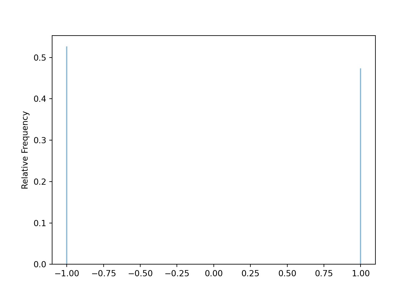
w.mean()## -0.05257894736842105For each simulated value, compute the squared deviation from the mean.
(w - w.mean()) ** 2| Index | Result |
|---|---|
| 0 | 0.8976066509695291 |
| 1 | 0.8976066509695291 |
| 2 | 1.1079224404432133 |
| 3 | 0.8976066509695291 |
| 4 | 1.1079224404432133 |
| 5 | 1.1079224404432133 |
| 6 | 0.8976066509695291 |
| 7 | 1.1079224404432133 |
| 8 | 1.1079224404432133 |
| ... | ... |
| 37999 | 0.8976066509695291 |
Summarize the squared deviations.
((w - w.mean()) ** 2).tabulate()| Value | Frequency |
|---|---|
| 0.8976066509695291 | 19999 |
| 1.1079224404432133 | 18001 |
| Total | 38000 |
Approximate the variance by computing the average squared deviation.
((w - w.mean()) ** 2).mean(), w.var()## (0.9972354542936285, 0.9972354542936285)Variance is also equal to the average of the squared values of \(W\) minus the square of the average value of \(W\).
(w ** 2).mean() - (w.mean()) ** 2## 0.9972354542936288The standard deviation is the square root of the variance.
sqrt(w.var()), w.sd()## (0.9986167704848685, 0.9986167704848685)Definition 5.3 The variance of a random variable \(X\) is \[\begin{align*} \textrm{Var}(X) & = \textrm{E}\left(\left(X-\textrm{E}(X)\right)^2\right)\\ & = \textrm{E}\left(X^2\right) - \left(\textrm{E}(X)\right)^2 \end{align*}\] The standard deviation of a random variable is \[\begin{equation*} \textrm{SD}(X) = \sqrt{\textrm{Var}(X)} \end{equation*}\]
Variance is, roughly, the long run average squared deviation from the mean. We square the deviations because when measuring distance from the mean it doesn’t matter if a value is above or below the mean. For example, a value that is 3 units above the mean has the same squared deviation as a value that is 3 units below the mean (\(3^2 = (-3)^2\)). You might think, why not just consider the absolute value of the deviations? It turns out that squaring leads to nicer mathematical properties126.
Standard deviation measures, roughly, the long run average distance from the mean. The measurement units of the standard deviation are the same as for the random variable itself.
The definition \(\textrm{E}((X-\textrm{E}(X))^2)\) represents the concept of variance. However, variance is usually computed using the following equivalent but slightly simpler formula.
\[ \textrm{Var}(X) = \textrm{E}\left(X^2\right) - \left(\textrm{E}\left(X\right)\right)^2 \]
That is, variance is the expected value of the square of \(X\) minus the square of the expected value of \(X\). The above formula basically allows us to subtract \(\textrm{E}(X)\) once rather than subtracting it from each value. The expected value of the square, \(\textrm{E}(X^2)\), can be computed with LOTUS.
In some cases, we have the expected value and variance and we want to compute \(\textrm{E}(X^2)\). Rearranging the above formula yields
\[ \textrm{E}\left(X^2\right) = \textrm{Var}(X) + \left(\textrm{E}\left(X\right)\right)^2 \]
We will see that variance has many nice theoretical properties. Whenever you need to compute a standard deviation, first find the variance and then take the square root at the end.
Example 5.12 Continuing with roulette, Nadja bets $1 on number 7. If the wheel lands on 7, Nadja wins her bet back plus an additional $35; otherwise she loses the money she bet. Let \(X\) be Nadja’s net winnings (net of the initial bet of $1.)
- Find the distribution of \(X\).
- Compute \(\textrm{E}(X)\).
- How do the expected values of the two $1 bets — bet on black versus bet on 7 — compare? Explain what this means.
- Are the two $1 bets — bet on black versus bet on 7 — identical? If not, explain why not.
- Before doing any calculations, determine if \(\textrm{SD}(X)\) is greater than, less than, or equal to \(\textrm{SD}(W)\). Explain.
- Compute \(\textrm{Var}(W)\) and \(\textrm{SD}(W)\).
- Which $1 bet — betting on black or betting on 7 — is “riskier”? How is this reflected in the standard deviations?
Solution. to Example 5.12
Show/hide solution
Assuming the wheel is equally likely to land on any of the 38 spaces, Nadja wins with probability 1/38 in which case her net winnings are 35 dollars; otherwise, her net winnings are \(-1\) dollar.
\(x\) \(p_X(x)\) -1 37/38 \(\approx\) 0.9737 35 1/38 \(\approx\) 0.0263 Use the definition of expected value of a discrete random variable. \[ \textrm{E}(X) = (-1)(37/38) + (35)(1/38) = -2/38 \approx -0.05 \]
The two expected values are the same. If Guillermo makes many $1 bets on black and Nadja makes many $1 bets on 7 then each will have long run average losses of about 5 cents per bet.
No, these are very different bets even though their expected values are the same. Guillermo wins about half the time, but his winnings are small. Nadja is much less likely to win, but when she does she wins big.
\(\textrm{SD}(X)\) is greater than \(\textrm{SD}(W)\). The mean is the same in both cases, but \(X\) can take values that are about 35 units away from the mean, so the average distance from the mean will be greater for \(X\) than for \(W\).
We use the computational formula. \[ \textrm{Var}(X) = E(X^2) - (\textrm{E}(X))^2 = \left[(-1)^2(37/38) + (35)^2(1/38)\right] - (-2/38)^2 \approx 33.2 \] So \(\textrm{SD}(X) = \sqrt{33.2} = 5.76\) dollars.
Betting on 7 is riskier; it’s less likely to win, but when it does the winnings are big. The riskier bet has the larger standard deviation.
The definition of variance is the same for discrete and continuous random variables. But remember that for continuous random variables expected values are computed via integration.
Example 5.13 Let \(X\) be a Uniform(\(a\), \(b\)) distribution.
- First, suppose \(X\) has a Uniform(0, 1) distribution. Make a ballpark estimate of the standard deviation.
- Compute \(\textrm{SD}(X)\) if \(X\) has a Uniform(0, 1) distribution.
- Now suggest a rough formula for the standard deviation for the general Uniform(\(a\), \(b\)) case.
- Compute \(\textrm{SD}(X)\) if \(X\) has a Uniform(\(a\), \(b\)) distribution.
Solution. to Example 5.13
Show/hide solution
- The expected value is 0.5. The deviations from the mean range from 0 (corresponding to a value of 0.5) to 0.5 (corresponding to a value of 0 or 1). Since the \(X\) values are uniformly distributed, the absolute deviations will also be uniformly distributed between 0 and 0.5. Therefore, we might guess that the average deviation from the mean is around 0.25.
- We computed \(E(X^2) = 1/3\) using LOTUS in Example 5.8. \(\textrm{Var}(X) = \textrm{E}(X^2) - (\textrm{E}(X))^2 = 1/3 - (1/2)^2 = 1/12\). \(\textrm{SD}(X) = 1/\sqrt{12}\approx 0.289\). The standard deviation isn’t quite 0.25 because squaring then averaging then taking the square root isn’t the same as just averaging the deviations. But 0.25 is not that far off.
- In general, the deviations range from 0 to \((b-a)/2\) (half the length of the interval), so we might guess the standard deviation is \((b-a)/4\)
- The pdf of \(X\) is \(f_X(x) = \frac{1}{b-a}, a<x<b\). Compute \(\textrm{E}(X^2)\) using LOTUS. \[ \textrm{E}(X^2) = \int_a^b x^2 \left(\frac{1}{b-a}\right)dx = \frac{x^3}{3(b-a)}\Bigg|_a^b = \frac{b^3 - a^3}{3(b-a)} \] Then, after some algebra, \[ \textrm{Var}(X) = \textrm{E}(X^2) - (\textrm{E}(X))^2 = \frac{b^3 - a^3}{3(b-a)} - \left(\frac{a+b}{2}\right)^2 = \frac{(b-a)^2}{12} \] The standard deviation is \[ \textrm{SD}(X) = \frac{b- a}{\sqrt{12}} \approx 0.289 (b-a) \] So our guess of 0.25 times the length of the interval was not too far off. Thinking of variability just in terms of the overall range of values, it makes sense that the standard deviation should depend on the length of the interval. That is, the standard deviation should only depend on \(a\) and \(b\) through their difference \(b-a\).
Example 5.14 The plots below summarize hypothetical distributions of quiz scores in six classes. All plots are on the same scale. Each quiz score is a whole number between 0 and 10 inclusive.
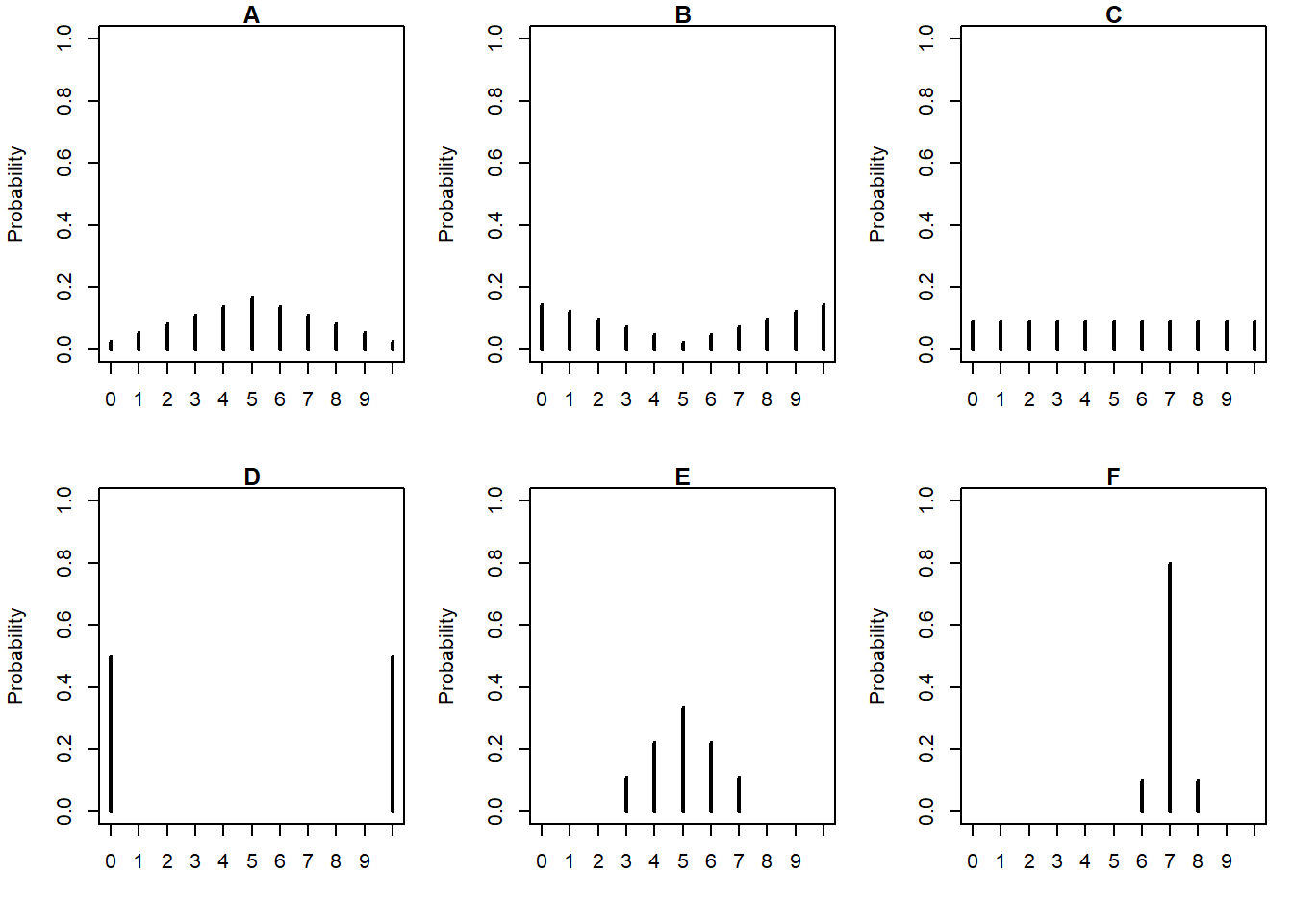
- Donny Dont says that C represents the smallest SD, since there is no variability in the heights of the bars. Do you agree that C represents “no variability? Explain.
- What is the smallest possible value the SD of quiz scores could be? What would need to be true about the distribution for this to happen? (This scenario might not be represented by one the plots.)
- Without doing any calculations, arrange the classes in order based on their SDs from smallest to largest.
- In one of the classes, the SD of quiz scores is 5. Which one? Why?
- Is the SD in F greater than, less than, or equal to 1? Why?
- Provide a ballpark estimate of SD in each case.
Solution. to Example 5.14
Show/hide solution
- We disagree with Donny. SD measures variability of the values of the variable, not their probabilities. If we were to simulate values according to the distribution in C, we would observe some 0s, some 1s, some 2s, all the way through some 10s (with roughly equal frequency). So there would certainly be variability in the values of the variable. Remember that values of the variable are along the horizontal axis, so SD measures average distance from the mean horizontally.
- The smallest possible value of SD is 0, which occurs only if the random variable is a constant (with probability 1). In this context, if every student had the same quiz score, e.g., if 100% of students scored an 8, then the SD would be 0. The distribution plot would have a single spike at a single value.
- Remember that values of the variable are along the horizontal axis, so SD measures average distance from the mean horizontally. The distribution in F represents the smallest SD. The mean is 7, most of the scores are 7, and some of the scores are only 1 unit of from the mean. In all other situations, the probability that the random variable is equal to its mean is smaller, and the probability that the random variables takes a value more than 1 unit away from its mean is larger than in F. Also, in all other situations the mean is 5, so the smallest SD occurs where the values tend to be close to 5, and the largest occurs where the values tend to be far from 5. In order from smallest to largest SD: F, E, A, C, B, D.
- D. In D, the score takes values 0 and 10 with probability 0.5. The mean is 5, and all deviations are 5 units away from the mean, so the SD will be 5.
- Less than 1. Don’t forget that there is a high probability of a deviation of 0 in this case. So the average deviation will be somewhere between 0 and 1.
- Some of these are harder than others. In E, many values are 0 units away from mean, many values are 1 unit away, and some values are 2. So the SD in E is maybe around 1. In C, there are values that are 0 units away, and about as many values that are each 1, 2, 3, 4, and 5 units away; we might expect SD to be around 2.5. But remember, while considering average distance helps intuition, SD is the square root of the average squared distance127. The actual values are: F = 0.45, E = 1.15, A = 2.4, C = 3.1, B = 3.7, D = 5.
Variance and standard deviation can not be negative. \(\textrm{Var}(X) = 0\) if and only if \(X\) is constant with probability 1, i.e., \(\textrm{P}(X = \textrm{E}(X)) = 1\).
Example 5.15 Let \(X\) have an Exponential(1) distribution. Make a ballpark estimate for \(\textrm{SD}(X)\), and then compute it.
Solution. to Example 5.15
Show/hide solution
It’s hard to make an estimate since \(X\) is continuous and the distribution is asymmetric, but we should at least get an idea of what might be a reasonable value. The mean is 1. The highest density occurs near 0, where values are about 1 unit away from the mean. But there is a high percentage of values that are less than 1 unit away from the mean. While there can be some extreme values, most of the values of \(X\) are at most 4, so at most 3 units above the mean. We might guess a SD of around 1. In particular, a guess of 2 would seem too high, since the only values that are more than 2 SDs above the mean are the \(X\) values that are greater than 3, and this is a relatively small percentage of values. A guess too close to 0 would be unreasonable because of the high density near 0 of values that are 1 unit below the mean.
We did all the hard work already: in Example 5.3 we found \(\textrm{E}(X) = 1\) and in Example 5.9 we found \(\textrm{E}(X^2) = 1\). Therefore, \(\textrm{Var}(X) = \textrm{E}(X^2) - \textrm{E}(X)^2 = 2 - (1)^2 = 1\) and \(\textrm{SD}(X) = 1\).
X = RV(Exponential(1))

X.sim(10000).sd()
## 0.99376613437331475.3.1 Standardization
Standard deviation provides a “ruler” by which we can judge a particular realized value of a random variable relative to the distribution of values. This idea is particularly useful when comparing random variables with different measurement units but whose distributions have similar shapes.
Recall Example 2.53 where we assumed SAT scores have, approximately, a Normal distribution with a mean of 1050 and a standard deviation of 200, and ACT scores have, approximately, a Normal distribution with a mean of 21 and a standard deviation of 5.5. Darius’s score of 1500 on the SAT was 2.25 standard deviations above the mean, relatively better than Alfred’s score of 31 on the ACT which was 1.82 above the mean.
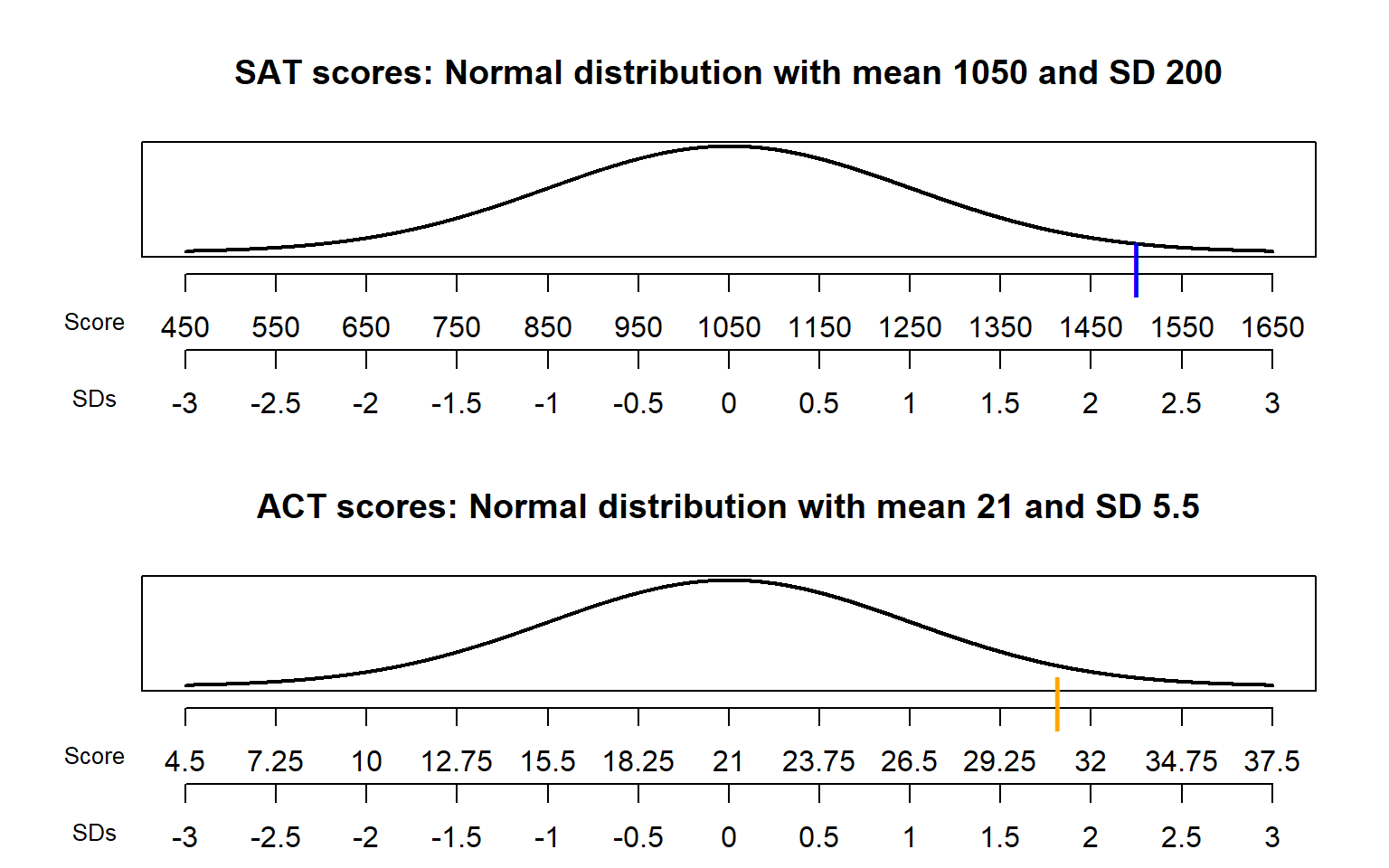
Figure 5.3: Comparison of the Normal distributions in Example 2.53. The blue mark indicates Darius’s SAT score and the orange mark indicates Alfred’s ACT score.
Consider the plot for SAT scores in Figure 5.3. There are two scales on the variable axis: one representing the actual measurement units, and one representing “standardized units”. In the standardized scale, values are measured in terms of standard deviations away from the mean:
- The mean corresponds to a value of 0.
- A one unit increment on the standardized scale corresponds to an increment equal to the standard deviation in the measurement unit scale.
For example, each one unit increment in the standardized scale corresponds to a 200 point increment in the measurement unit scale for SAT scores, and a 5.5 point increment in the measurement unit scale for ACT scores. An SAT score of 1250 is “1 standard deviation above the mean”; an ACT score of 10 is “2 standard deviations below the mean. Given a distribution, the more standard deviations a particular value is away from its mean, the more extreme or”unusual” it is.
Definition 5.4 If \(X\) is a random variable with expected value \(\textrm{E}(X)\) and standard deviation \(\textrm{SD}(X)\), then the standardized random variable is \[ Z = \frac{X - \textrm{E}(X)}{\textrm{SD}(X)} \]
For each outcome \(\omega\), the standardized value \(Z(\omega)\) measures how far the value \(X(\omega)\) is away from the expected value relative to the degree of variability of values of the random variable. The random variable \(X\) itself is measured in measurement units (feet, inches, dollars, etc), and the standardized random variable \(Z\) is measured in standardized units — “standard deviations away from the mean”.
Standardization — that is, subtracting the mean and dividing by the standard deviation — is a linear rescaling. Therefore, the shape of the distribution of the standardized random variable will be the same as the shape of the distribution of the original random variable. However, the possible values will be different, and so will the mean and standard deviation. Regardless of the original measurement units, a standardized random variable has mean 0 and standard deviation 1.
However, keep in mind that comparing standardized values is most appropriate for distributions that have similar shapes.
Example 5.16 For which distribution — Uniform(0, 1) or Exponential(1) — is it more unsual to see a value smaller than 0.15?
- Standardize the value 0.15 relative to the Uniform(0, 1) distribution.
- Standardize the value 0.15 relative to the Exponential(1) distribution.
- Donny Dont says: “For the Uniform(0, 1) distribution, a value of 0.15 is 1.2 standard deviations below the mean. For the Exponential(1) distribution, a value of 0.15 is 0.85 standard deviations below the mean. So a value smaller than 0.15 is more unusual for a Uniform(0, 1) distribution, since there it’s more standard deviations below the mean.” Do you agree with his conclusion? Explain.
- How can you answer the original question in the setup?
- The value 0.15 is what percentile for a Uniform(0, 1) distribution?
- The value 0.15 is what percentile for an Exponential(1) distribution?
- For which distribution — Uniform(0, 1) or Exponential(1) — is it more unsual to see a value smaller than 0.15?
Solution. to Example 5.16
Show/hide solution
- The mean of the Uniform(0, 1) distribution is 0.5, and the standard deviation is \(1/\sqrt{12}\approx 0.289\). (See Example 5.13.) The standardized value for 0.15 is \((0.15 - 0.5)/(1/\sqrt{12})\approx -1.2\). Relative to the Uniform(0, 1) distribution, a value of 0.15 is about 1.2 SDs below the mean.
- The mean of the Exponential(1) distribution is 1, and the standard deviation is 1. (See Example 5.15.) The standardized value for 0.15 is \((0.15 - 1)/1 = -0.85\). Relative to the Exponential(1) distribution, a value of 0.15 is 0.85 SDs below the mean.
- Donny’s statements about the standardized values are fine, but his conclusion is not. The distributions here have different shapes, so for example, 1 SD below the mean does not correspond to the same percentile for the two distributions.
- We can see what percentile a value of 0.15 represents for each distribution.
- The Uniform(0, 1) cdf is \(F(x) = x, 0<x<1\), so \(F(0.15) = 0.15\). For the Uniform(0, 1) distribution, the probability of a value smaller than 0.15 is 0.15; 0.15 is the 15th percentile.
- The Exponential(1) cdf is \(F(x) = 1-e^{-x}, x>0\), so \(F(0.15) = 1-e^{-0.15} \approx 0.14\). For the Exponential(1) distribution, the probability of a value smaller than 0.15 is 0.14; 0.15 is the 14th percentile.
- While it’s close, it is a little less likely to see a value smaller than 0.15 for the Exponential(1) distribution than for the Uniform(0, 1) distribution. Notice that this is true despite the fact that the standardized value for 0.15 is more standard deviations below the mean for the Uniform(0, 1) distribution than for the Exponential(1) distribution.
Standardization is useful when comparing random variables with different measurement units but whose distributions have similar shapes. However, standardized values are only based on two features of a distribution — mean and standard deviation — rather than the complete pattern of variability. Distributions with different shapes have different patterns of variability. Therefore, when comparing distributions with different shapes, it is better to compare percentiles rather than standardized values to determine what is “extreme” or “unusual”.
See Figure 5.4 for an illustration. The figure displays the cdf of each of the Normal(0, 1), Exponential(1), and Uniform(0, 1) distributions as a function of standardized values. Notice how the standardized values correspond to different percentiles for the three distributions. In particular, a standardized value of 0 corresponds to the median for the Normal(0, 1) and Uniform(0, 1) distributions, but it represents the 63rd percentile for the Exponential(1) distribution. For another example, a standardized value of \(-0.95\) corresponds to:
- a value of \(-0.95\) from the Normal(0, 1) distribution, which is about the 17th percentile
- a value of \(1-0.95(1) = 0.05\) from the Exponential(1) distribution, which is about the 5th percentile
- a value of \(0.5-0.95(1/\sqrt{12}) = 0.226\) from the Uniform(0, 1) distribution, which is about the 23rd percentile.
Among these three distributions, a value 0.95 SDs below the mean is most extreme for the Exponential(1) distribution and least extreme for the Uniform(0, 1) distribution.
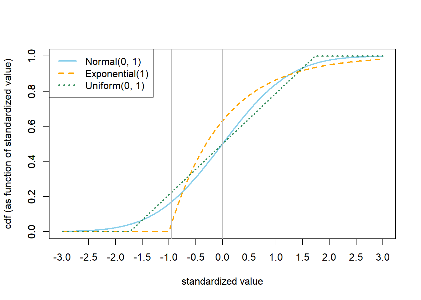
Figure 5.4: Comparison of cdf, as a function of standardized value, for the Normal(0, 1), Exponential(1), and Uniform(0, 1) distributions.
Any random variable can be standardized, but keep in mind that just how extreme any particular standardized value is depends on the shape of the distribution. In general, standardization is most natural for random variables that follow a Normal distribution, where percentiles follow the empirical rule discussed in Section 2.10.2.
5.3.2 Probability inequalitlies
The distribution of a random variable is a complete description of its pattern of variability. Knowing the distribution of a random variable allows you to compute the probability of any event involving it, but the full distribution is often unavailable or difficult to obtain. However, certain summary characteristics, like the mean or standard deviation, might be available. What can we say about a distribution based on only information about its mean or standard deviation?
5.3.2.1 Markov’s inequality
Example 5.17 According to 2019 data from the U.S. Census Bureau, the mean128 annual income for U.S. households is about $100,000. Suppose that you know nothing else about the distribution of income, other than income can’t be negative. What can you say about the percent of households with incomes of at least $1 million?
- Can 100% of households have income of at least $1 million?
- Can 50% of households have income of at least $1 million?
- What is the largest possible percentage of households with incomes of at least $1 million?
Solution. to Example 5.17
Show/hide solution
- No, if 100% of households have incomes of least 1 million, then the mean must be at least 1 million. If every household had an income of exactly 1 million, then the mean would be 1 million.
- No, if 50% of households have incomes of at least 1 million, then the mean must be at least 500,000. Even if 50% of households have incomes of exactly 1 million and the rest have incomes of 0 (the smallest possible value), the mean would be 500,000.
- The idea is that if too many households have incomes above 1 million then the average can’t be 100,000. Classify each household as either having an income of at least 1 million or not. The mean will be smallest in the extreme case where each household has an income of either 1 million or 0; allowing other values will just pull the mean up. In this extreme scenario, let \(p\) be the proportion of households with an income of 1 million. Then the mean is \(1000000p + 0(1-p) = 1000000p\), and setting it equal to 100000 yields \(p=0.1\). Therefore, given a mean of $100,000 it is theoretically possible for 10% of households to have incomes of at least $1 million. But 10% is the maximum possible percentage; if more than 10% of households have incomes above $1 million, than the mean would be strictly greater than $100,000. Knowing only that the mean is 100,000, all we can say is that between 0% and 10% of households have incomes of at least $1 million.
The scenario corresponding to 10% in the previous example is hypothetical, and in reality far fewer than 10% of U.S. households have incomes of at least $1 million. (Only about 10% of households have incomes above $200,000, so the percentage of households with incomes above $1 million is much smaller than 10%.) However, the scenario is theoretically possible so we must account for it. We can’t do any better based on knowing just the mean alone without any additional information about the distribution of incomes.
The previous example illustrates Markov’s inequality.
Theorem 5.1 (Markov's inequality) For any random variable \(X\) and any constant \(c>0\) \[ \textrm{P}(|X|\ge c) \le \frac{\textrm{E}(|X|)}{c}. \] In particular, if \(\textrm{P}(X\ge0)=1\) then \(\textrm{P}(X > c) \le \textrm{E}(X)/c\).
The idea behind Markov’s inequality is that large values pull the mean up, so given a fixed value of the mean there is a limit on the probability that the random variable takes large values. The proof uses the same strategy as Example 5.17. Each value of \(|X|\) is either at least \(c\) or not. Consider the extreme situation where each value of \(|X|\) is either \(c\) or 0. That is, define the random variable \(Y=c\textrm{I}\{|X|\ge c\}\). Then \(|X|\ge Y\); if \(|X|\ge c\) then \(Y=c\); if \(|X|<c\) then \(Y=0\). Therefore \(\textrm{E}(|X|)\ge \textrm{E}(Y)\) and \[ \textrm{E}(|X|)\ge\textrm{E}(Y) = \textrm{E}(c\textrm{I}\{|X|\ge c\}) = c\textrm{P}(|X| \ge c). \] Divide by \(c>0\) to get the result.
Think of \(c\) as a large value in the measurement units of the random variable, so Markov’s inequality provides a very crude upper bound on the probability that \(X\) takes extreme values in the absolute sense. Probabilities like \(\textrm{P}(|X| \ge c)\) are called “tail probabilities” because they depend on the “tail” of the distribution which describes the pattern of variability for extreme values.
We can also express Markov’s inequality in relative terms. If \(X\ge 0\), then for any constant \(k\) \[ \textrm{P}(X \ge k \textrm{E}(X)) \le \frac{\textrm{E}(X)}{k\textrm{E}(X)} = \frac{1}{k} \] Think of \(k\) as a multiplier: what is the probability that the random variable takes a value at least \(k\) times larger than the average value? Markov’s inequality says that at most \(1/k\) of values are at least \(k\) times greater than the mean. For example, at most 1/2 of values are at least 2 times as large as the mean; at most 1/3 of values are at least 3 times as large as the mean; etc.
Example 5.18 Suppose \(X\) is a random variable with an Exponential(1) distribution. What does Markov’s inequality say about \(\textrm{P}(X > 5)\)? How does this compare to the true probability?
Solution. to Example 5.18
Show/hide solution
The mean of an Exponential(1) distribution is 1, so Markov’s inequality says \[ \textrm{P}(X\ge 5) \le \frac{\textrm{E}(X)}{5} = \frac{1}{5} = 0.2. \] The true probability is \(e^{-5}\approx 0.0067\). The true probability is about 30 times smaller than the bound provided by Markov’s inequality. Markov’s inequality only uses the fact the mean is 1; it provides a bound that works for any distribution with a mean of 1. But it is not guaranteed to work well for any particular distribution.
The upper bound provided by Markov’s inequality often grossly overestimates the tail probability. However, without further information, we cannot rule out the extreme but theoretically possible case in which the tail probability \(\textrm{P}(|X|\ge c)\) is equal to the upper bound \(\textrm{E}(|X|)/c\). Markov’s inequality provides a bound that works for any distribution with a given mean, but it is not guaranteed to work well for any particular distribution.
If the upper bound is so bad, how is Markov’s inequality useful? Think of reading a news article involving some numerical variable. The article might mention the mean, but have you ever read a news article that mentions the standard deviation? At best, you might get a range of “typical” values, maybe a percentile or two, or a graph if you’re really lucky. But in many situations, the mean might be all that is available, and Markov’s inequality at least tells you something about the distribution based on the mean alone (even if it doesn’t tell you much).
5.3.2.2 Chebyshev’s inequality
Markov’s inequality only relies on the mean, but it provides very rough bounds on tail probabilities. If we have more information, then we can do better. In particular, if we also know the standard deviation — which describes the overall degree of variability — then we can put better bounds on the probability that a random variable takes a value far from its mean.
Theorem 5.2 (Chebyshev's inequality) For any random variable \(X\) and any constant \(c>0\)
\[ \textrm{P}\left(|X-\textrm{E}(X)|\ge c\right)\le \frac{\textrm{Var}(X)}{c^2}. \]
Equivalently, for any constant \(z>0\), \[ \textrm{P}\left(\frac{|X-\textrm{E}(X)|}{\textrm{SD}(X)}\ge z\right)\le \frac{1}{z^2}. \]
The first version of Chebyshev’s inequality bounds the probability that a random variable is at least \(c\) measurement units away from its mean. The proof is an application of Markov’s inequality to the squared deviation random variable \(|X-\textrm{E}(X)|^2\): \[ \textrm{P}\left(|X-\textrm{E}(X)|\ge c\right) = \textrm{P}\left(|X-\textrm{E}(X)|^2\ge c^2\right) \le \frac{\textrm{E}\left(|X-\textrm{E}(X)|^2\right)}{c^2}= \frac{\textrm{Var}(X)}{c^2}. \]
Example 5.19 Continuing Example 5.17, suppose again that average annual income for U.S. households is about $100,000. Now assume the standard deviation of income is about $230,000. What can you say about the percent of households with incomes of at least $1 million?
Show/hide solution
We first need to relate the probability of interest to one that is of the form129 in Chebyshev’s inequality. An income of 1 million is 900,000 dollars above the mean of 100,000.
\[ \textrm{P}\left(X \ge 1000000\right) = \textrm{P}\left(X-100000\ge 900000\right) \le \textrm{P}\left(|X-100000|\ge 900000\right). \] Now use Chebyshev’s inequality with \(c=900000\), \(\textrm{E}(X) = 100000\), and \(\textrm{Var}(X) = 230000^2\). \[ \textrm{P}\left(X \ge 1000000\right) \le \textrm{P}\left(|X-100000|\ge 900000\right)\le \frac{230000^2}{900000^2} = 0.065. \]
Alternatively, a value of 1000000 is \(z=(1000000 - 100000) / 230000 = 3.91\) SDs above the mean, so the probability that the standardized random variable is at least 3.91 is less than \(1/3.91^2\approx 0.065\).
With information about the mean and standard deviation, we can say that at most 6.5% of households have income above $1 million. This is still probably a vast overestimate, but it does improve on the bound of 10% from Markov’s inequality.
The bound in Markov’s inequality is on the order of \(1/c\) and the bound in Chebyshev’s inequality is on the order of \(1/c^2\). Therefore, Chebyshev’s inequality usually provides a tighter bound, but you need to know the standard deviation in order to use it.
The second version of Chebyshev’s inequality follows by taking \(c = z\textrm{SD}(X)\) in the first version. The second version bounds the probability that a random variable is at least \(z\) standard deviations away from its mean. Chebyshev’s inequality says that for any distribution, the probability that the random variable takes a value within \(z\) SDs of its mean is at least \(1 - 1 / z^2\). For any distribution,
- (\(z = 2\).) At least 75% of values fall within 2 standard deviations of the mean.
- (\(z = 3\).) At least 88.9% of values fall within 3 standard deviations of the mean.
- (\(z = 4\).) At least 93.75% of values fall within 4 standard deviations of the mean.
- (\(z = 5\).) At least 96% of values fall within 5 standard deviations of the mean.
- (\(z = 6\).) At least 97.2% of values fall within 6 standard deviations of the mean.
- and so on, for different values of \(z\).
The complementary probabilities: For any distribution,
- (\(z = 2\).) At most 25% of values fall more than 2 standard deviations away from the mean.
- (\(z = 3\).) At most 11.1% of values fall more than 3 standard deviations away from the mean.
- (\(z = 4\).) At most 6.25% of values fall more than 4 standard deviations away from the mean.
- (\(z = 5\).) At most 4% of values fall more than 5 standard deviations away from the mean.
- (\(z = 6\).) At most 2.8% of values fall more than 6 standard deviations away from the mean.
- and so on, for different values of \(z\).
This universal “empirical rule” works for any distribution, but will tend to be very conservative when applied to any particular distribution.
In short, Chebyshev’s inequality says that if a value is more than a few standard deviations away from the mean then it is a fairly extreme value, regardless of the shape of the distribution.
Example 5.20 Let \(X\) be a random variable with an Exponential(1) distribution. What does Chebyshev’s inequality say about \(\textrm{P}(X > 5)\)? How does this compare to the bound from Markov’s inequality? To the true probability?
Solution. to Example 5.20
Show/hide solution
Both the mean and the standard deviation of an Exponential(1) distribution are 1. A value of 5 is \((5-1)/1=4\) units above the mean. Chebyshev’s inequality says that the probability that a value is at least 4 units away from the mean is at most \(1/4^2 = 0.0625\). This bound is 3 times smaller than 0.2, the bound from Markov’s inequality. It’s still not close to the true probability of \(0.0067\), but at least it’s an improvement over Markov’s inequality.
Another situation where bounds like Markov’s or Chebyshev’s inequality are useful is in proofs. Many theorems in probability consider what happens in the long run. For example, various results say certain probabilities approach 0 in the long run. (The law of large numbers is of this form.) To prove such theorems, you don’t necessarily need to compute the probabilities to show they approach 0. It is enough to show that some rough upper bound on the probability converges to 0.
You might think that the expected value doesn’t tell us anything about the degree of variability. But knowing the expected value does put a very rough limit on the probability that the random variable takes very large values. We’ll discuss this idea when we cover Markov’s inequality in Section 5.3.2.1. In any case, the expected value alone tells us very little about the degree of variability.↩︎
Think Pythagorean theorem: it’s \(a^2 + b^2 = c^2\). On the other hand, the triangle inequality says \(|a + b| \le |a| + |b|\).↩︎
It can be shown that \(\textrm{E}(|X-\textrm{E}(X)|)\le \textrm{SD}(X)\)↩︎
The mean is closer to $98,000 but we’re rounding to simplify a little. It is often more appropriate to consider median income, rather than mean income. The median annual income for U.S. households in 2019 was about $69,000.↩︎
The form we have stated bounds the probability that \(X\) is far away from the mean. There are also one-sided Chebyshev’s inequalities that bound the probability that \(X\) is far above (or below) its mean. If we recognize that \(X\) in this example can’t be 900000 units below its mean, a one-sided Chebyshev’s inequality yields a bound of \((1/(1+900000/230000))^2\approx 0.042\).↩︎