2.10 Standard deviation
The long run average value is just one feature of a distribution. Random variables vary, and the distribution describes the entire pattern of variability. We can summarize this degree of variability by listing some percentiles (10th, 25th, 50th, 75th, 90th, etc); the more percentiles we provide the clearer the picture, but the less of a summary. It is also convenient to measure overall degree of variability in a single number.
Consider again a random variable \(X\) that follows a Normal(30, 10) distribution (like Regina’s arrival time in one case of the meeting problem).
X = RV(Normal(30, 10))

x = X.sim(10000)
x| Index | Result |
|---|---|
| 0 | 24.959099114320566 |
| 1 | 24.061101514013824 |
| 2 | 43.92798251188586 |
| 3 | 54.75761964329468 |
| 4 | 45.388680820721945 |
| 5 | 20.771988728380812 |
| 6 | 13.411326019601923 |
| 7 | 27.173361726569002 |
| 8 | 24.504191323306074 |
| ... | ... |
| 9999 | 35.4148287003167 |
x.plot()
Normal(30, 10).plot() # plot the density curve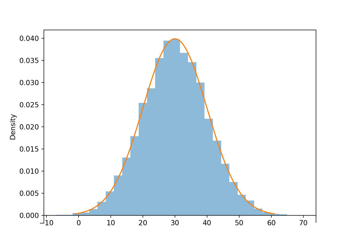
x.mean()## 29.981660607093755The simulation results suggest that 30 is the balance point of the distribution, and 30 seems like a reasonable value of the long run average based on average of the simulated values. It is. Any Normal distribution has two parameters, one of which is the mean, a.k.a. long run average value. A Normal(30, 10) distribution is a Normal distribution with mean 30 and standard deviation 10.
Standard deviation is a measure of overall degree of variability. While the long run average of \(X\) is 30, the values vary about that average.
Many values are close to the average, but some are farther away. The standard deviation measures, roughly, the average distance of the values from their mean. Calling x.sd() will compute the standard deviation of the simulated values in x; we see that it’s about 10.
x.sd()## 10.048794632212013Roughly, standard deviation measures the average distance from the mean. First, for each simulated value compute its absolute distance from the mean.
abs(x - x.mean())| Index | Result |
|---|---|
| 0 | 5.022561492773189 |
| 1 | 5.92055909307993 |
| 2 | 13.946321904792104 |
| 3 | 24.775959036200927 |
| 4 | 15.40702021362819 |
| 5 | 9.209671878712943 |
| 6 | 16.570334587491832 |
| 7 | 2.8082988805247524 |
| 8 | 5.477469283787681 |
| ... | ... |
| 9999 | 5.4331680932229425 |
Then average these distances.
abs(x - x.mean()).mean()## 8.021453884342586Unfortunately, the above calculation yields roughly 8 rather than the value of roughly 10 that x.sd() returns.
The above calculation illustrates the concept of standard deviation as average distance from the mean, but the actual calculation of standard deviation is a little more complicated.
Technically, you must first square all the distances and then average; the result is the variance.
The standard deviation is then the square root of the variance.
\[\begin{align*} \text{Variance of } X & = \text{Average of } [(X - \text{Average of X})^2]\\ \text{Standard deviation of } X & = \sqrt{\text{Variance of } X} \end{align*}\]
The standard deviation is measured in the measurement units of the random variable. For example, if the random variable is measured in inches, then standard deviation is also measured in inches, while variance is measured in square-inches. We will see the theory of variance and standard deviation later.
The following code shows the “long way” of computing standard deviation. First, find the squared distance between each simulated value and the mean.
(x - x.mean()) ** 2 | Index | Result |
|---|---|
| 0 | 25.226123948688045 |
| 1 | 35.05301997465145 |
| 2 | 194.49989467208405 |
| 3 | 613.8481461635064 |
| 4 | 237.37627186314765 |
| 5 | 84.81805611355598 |
| 6 | 274.5759883414281 |
| 7 | 7.8865426023565774 |
| 8 | 30.002669754837527 |
| ... | ... |
| 9999 | 29.519315529215824 |
Then average the squared distances to obtain the variance.
The average is computed in the usual way: sum all the values and divide by the number of values82.
But now each value included in the average is the squared deviation of x from the mean, rather than the value of x itself.
((x - x.mean()) ** 2).mean()## 100.97827356037298Compare with
x.var()## 100.97827356037298Now take the square root to get the standard deviation.
The value is the same as the one returned by x.sd().
sqrt(((x - x.mean()) ** 2).mean())## 10.048794632212013Example 2.52 We’ll compare long run average and standard deviation for the Uniform(0, 60) distribution and the Normal(30, 10) distribution.
- Make an educated guess for the long run average value of a Uniform(0, 60) distribution.
- Will the standard deviation for a Uniform(0, 60) distribution be greater than, less than, or equal to 10, the standard deviation for a Normal(30, 10) distribution? Explain without doing any calculations.
- Make an educated guess for the standard deviation of a Uniform(0, 60) distribution.
Solution. to Example 2.52.
Show/hide solution
- It seems reasonable that the long run average value of a Uniform(0, 60) distribution is 30, the balance point of the distribution.
- While the Uniform(0, 60) and Normal(30, 10) distributions have the same mean of 30, the Uniform(0, 60) has a larger standard deviation than the Normal(30, 10) distribution. In comparison to a Normal(30, 10) distribution, a Uniform(0, 60) distribution will give higher probability to ranges of values near the extremes of 0 and 60, as well as lower probability to ranges of values near 30. Thus, there will be more values far from the mean of 30 and fewer values close, and so the average distance from the mean and hence standard deviation will be larger for the Uniform(0, 60) distribution than for the Normal(30, 10) distribution. So the standard deviation of a Uniform(0, 60) distribution will be greater than 10.
- In a Uniform(0, 60) distribution, values are “evenly spread” from 0 to 60, so distances from the mean are “evenly spread” from 0 (for 30) to 30 (for 0 and 60). We might expect the standard deviation — that is, the average distance from the mean — to be about 15, halfway between 0 and 30. It turns out that the standard deviation is about 17. While the “average distance” interpretation helps our conceptual understanding of standard deviation, the process of squaring the distances, then averaging, and then taking the square root makes guessing the actual value of standard deviation difficult.
RV(Normal(30, 10)).sim(10000).plot() # plot simulated values
Normal(0, 30).plot() # plot the theoretical density

RV(Uniform(0, 60)).sim(10000).plot() # plot simulated values
Uniform(0, 60).plot() # plot the theoretical density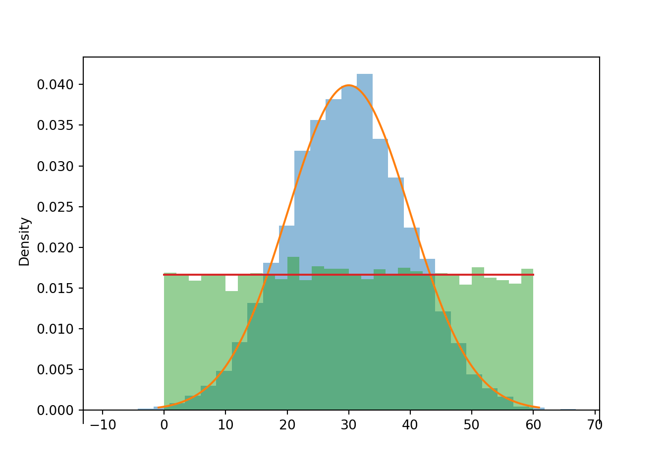
RV(Uniform(0, 60)).sim(10000).sd()## 17.199051294036152.10.1 Standardization
Standard deviation provides a “ruler” by which we can judge a particular realized value of a random variable relative to the distribution of values. This idea is particularly useful when comparing random variables with different measurement units but whose distributions have similar shapes.
Example 2.53 SAT scores have, approximately, a Normal distribution with a mean of 1050 and a standard deviation of 200. ACT scores have, approximately, a Normal distribution with a mean of 21 and a standard deviation of 5.5. Darius’s score on the SAT is 1500. Alfred’s score on the ACT is 31. Who scored relatively better on their test?
- Compute the deviation from the mean for Darius’s SAT score. How does this compare to the average deviation from the mean for SAT scores?
- Compute the deviation from the mean for Alfred’s ACT score. How does this compare to the average deviation from the mean for ACT scores?
- Who scored relatively better on their test?
Solution. to Example 2.53
Show/hide solution
- Darius’s score is \(1500-1050 = 450\) points above the mean SAT score. The average deviation of SAT scores from the mean is 200 points. So the deviation of Darius’s score from the mean is \(450/200 = 2.25\) times larger the average deviation.
- Alfred’s score is \(31-21 = 10\) points above the mean ACT score. The average deviation of ACT scores from the mean is 5.5 points. So the deviation of Alfred’s score from the mean is \(10/5.5 = 1.82\) times larger than the average deviation.
- Both scores are above average, but Darius’s is farther above average than Alfred’s. Both distributions are Normal, so the probability that an SAT score is greater than Darius’s is smaller than the probability that an ACT score is greater than Alfred’s. That is, Darius scored relatively better. See Figure 2.37.
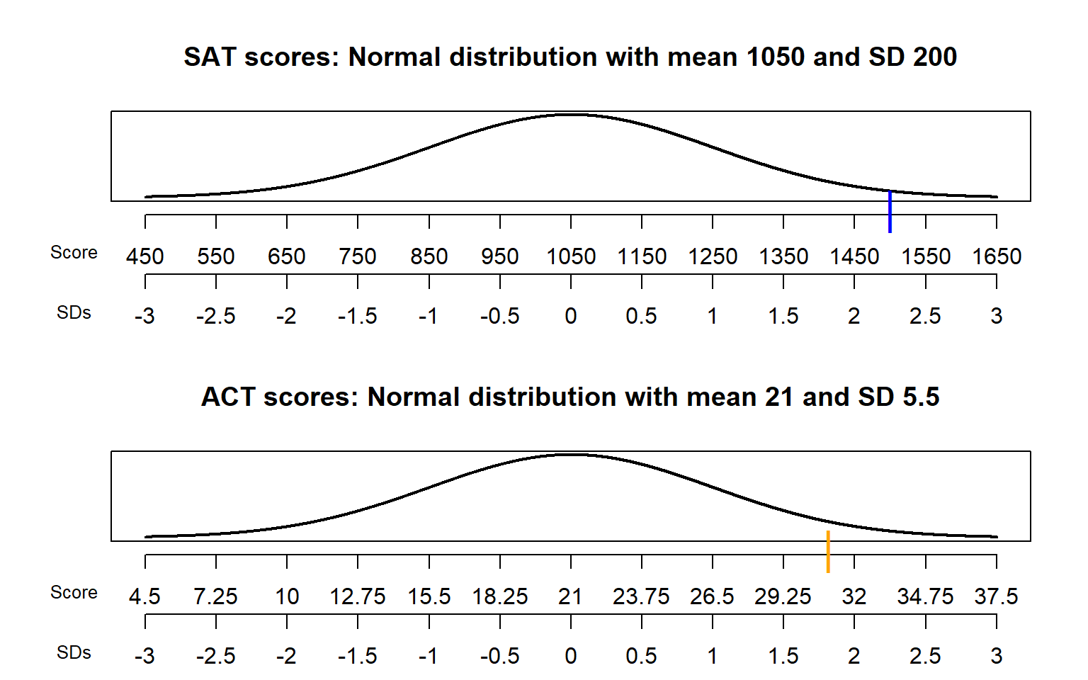
Figure 2.37: Comparison of the Normal distributions in Example 2.53. The blue mark indicates Darius’s SAT score and the orange mark indicates Alfred’s ACT score.
Standard deviation provides a “ruler” by which we can judge a particular realized value of a random variable relative to the distribution of values. Consider the plot for SAT scores in Figure 2.37. There are two scales on the variable axis: one representing the actual measurement units, and one representing “standardized units”. In the standardized scale, values are measured in terms of standard deviations away from the mean:
- The mean corresponds to a value of 0.
- A one unit increment on the standardized scale corresponds to an increment equal to the standard deviation in the measurement unit scale.
For example, each one unit increment in the standardized scale corresponds to a 200 point increment in the measurement unit scale for SAT scores, and a 5.5 point increment in the measurement unit scale for ACT scores. An SAT score of 1250 is “1 standard deviation above the mean”; an ACT score of 10 is “2 standard deviations below the mean”. Given a specific distribution, the more standard deviations a particular value is away from its mean, the more extreme or “unusual” it is.
The standardized value is
\[ \text{Standardized value} = \frac{\text{Value - Mean}}{\text{Standard deviation}} \]
Standardization — that is, subtracting the mean and dividing by the standard deviation — is a linear rescaling. Therefore, the shape of the distribution of the standardized random variable will be the same as the shape of the distribution of the original random variable. However, the possible values will be different, and so will the mean and standard deviation. Regardless of the original measurement units, a standardized random variable has mean 0 and standard deviation 1.
Standardization is useful when comparing random variables with different measurement units but whose distributions have similar shapes. However, standardized values are only based on two features of a distribution — mean and standard deviation — rather than the complete pattern of variability. Distributions with different shapes have different patterns of variability. Therefore, when comparing distributions with different shapes, it is better to compare percentiles rather than standardized values to determine what is “extreme” or “unusual”.
Any random variable can be standardized, but keep in mind that just how extreme any particular standardized value is depends on the shape of the distribution. Standardization is most natural for random variables that follow a Normal distribution.
2.10.2 Normal distributions and the empirical rule
Any Normal distribution follows the “empirical rule” which determines the percentiles that give a Normal distribution its particular bell shape. For example, for any Normal distribution the 84th percentile is about 1 standard deviation above the mean, the 16th percentile is about 1 standard deviation below the mean, and about 68% of values lie within 1 standard deviation of the mean. The table below lists some percentiles of a Normal distribution.
| Percentile | SDs away from the mean |
|---|---|
| 0.1% | 3.09 SDs below the mean |
| 0.5% | 2.58 SDs below the mean |
| 1% | 2.33 SDs below the mean |
| 2.5% | 1.96 SDs below the mean |
| 10% | 1.28 SDs below the mean |
| 15.9% | 1 SDs below the mean |
| 25% | 0.67 SDs below the mean |
| 30.9% | 0.5 SDs below the mean |
| 50% | 0 SDs above the mean |
| 69.1% | 0.5 SDs above the mean |
| 75% | 0.67 SDs above the mean |
| 84.1% | 1 SDs above the mean |
| 90% | 1.28 SDs above the mean |
| 97.5% | 1.96 SDs above the mean |
| 99% | 2.33 SDs above the mean |
| 99.5% | 2.58 SDs above the mean |
| 99.9% | 3.09 SDs above the mean |
The table only lists select percentiles. An even more compact version: For a Normal distribution
- 68% of values are within 1 standard deviation of the mean
- 95% of values are within 2 standard deviations of the mean
- 99.7% of values are within 3 standard deviations of the mean
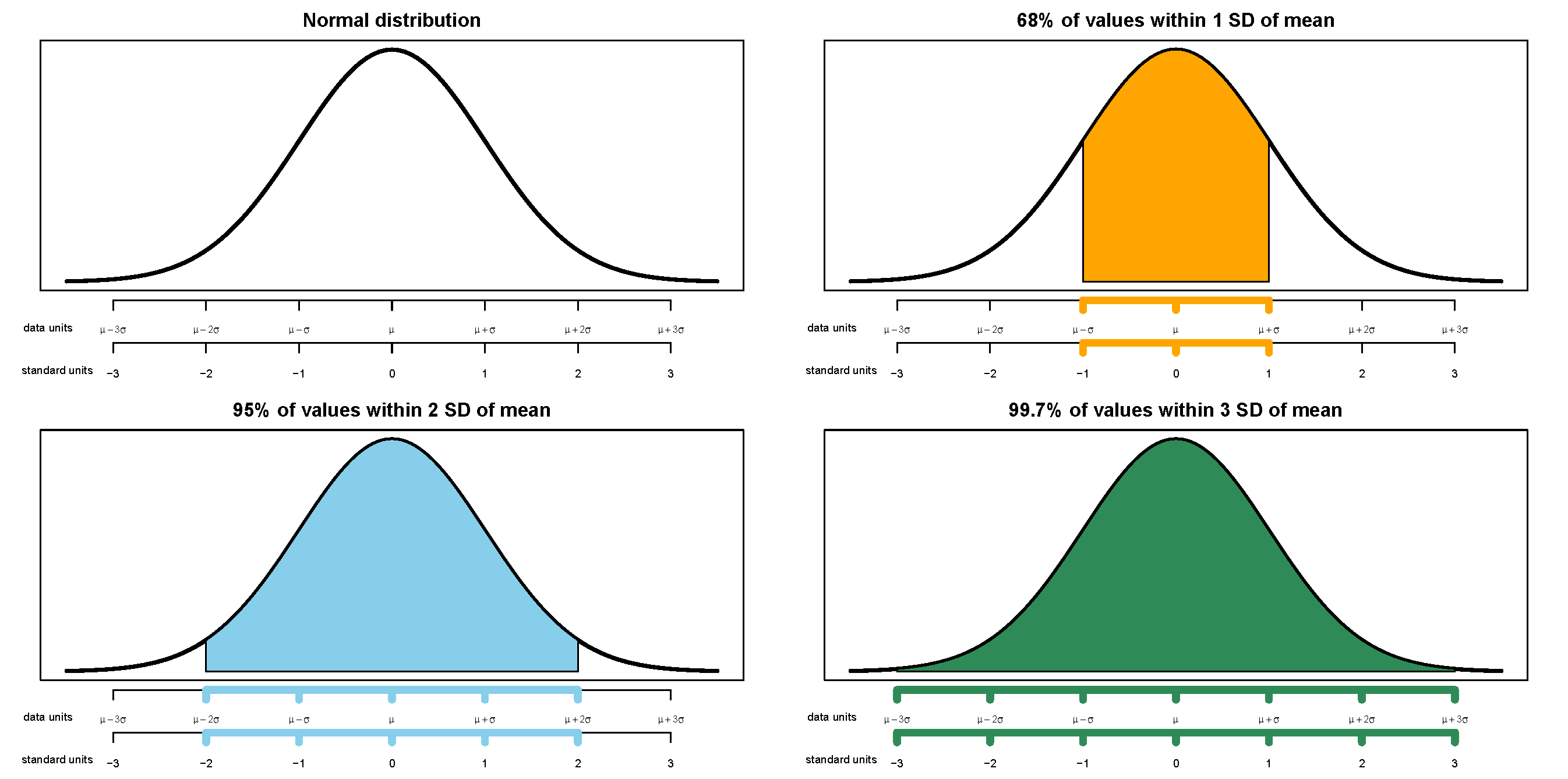
The “standard” Normal distribution is a Normal(0, 1) distribution, with a mean 0 and a standard deviation of 1. Notice how the empirical rule corresponds to the standard Normal spinner below.
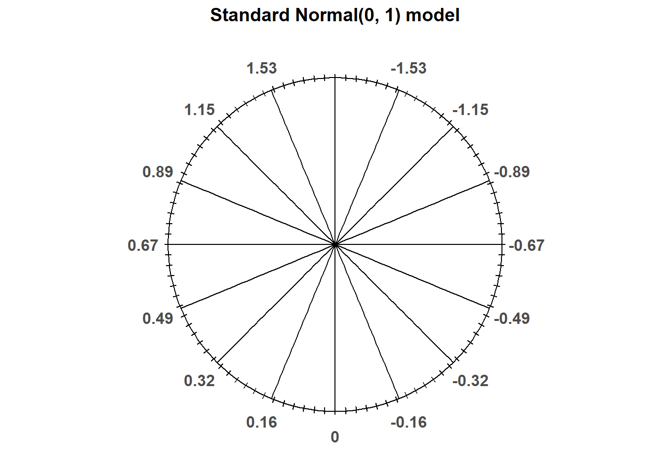
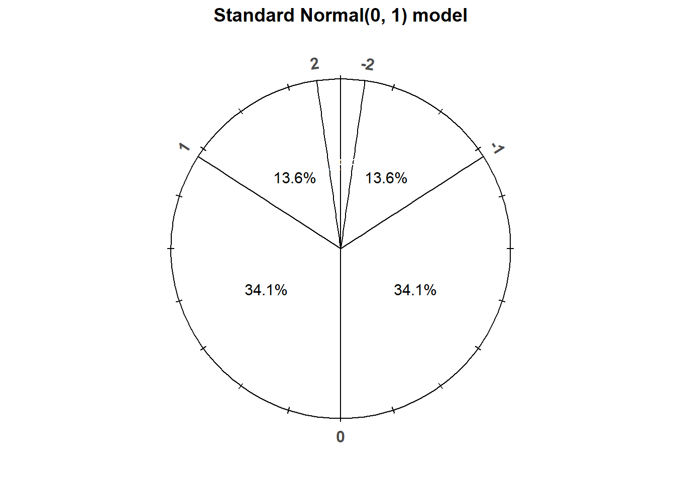
Figure 2.38: A “standard” Normal(0, 1) spinner. The same spinner is displayed on both sides, with different features highlighted on the left and right. Only selected rounded values are displayed, but in the idealized model the spinner is infinitely precise so that any real number is a possible outcome. Notice that the values on the axis are not evenly spaced.
If you have some familiarity with statistics, you might have seen a formula for standard deviation that includes dividing by one less than the number values (\(n-1\)). Dividing by \(n\) or \(n-1\) could make a difference in a small sample of data. However, we will always be interested in long run averages, and it typically won’t make any practical difference whether we divide by say 10000 or 9999.↩︎