6.3 Negative Binomial distributions
In a Binomial situation, the number of trials is fixed and we count the (random) number of successes. In other situations we perform trials until a certain number of successes occurs and we count the (random) number of trials
6.3.1 Geometric distributions
Example 6.10 Maya is a basketball player who makes 40% of her three point field goal attempts. Suppose that she attempts three pointers until she makes one and then stops. Let \(X\) be the total number of shots she attempts. Assume shot attempts are independent.
- Does \(X\) have a Binomial distribution? Why or why not?
- What are the possible values that \(X\) can take? Is \(X\) discrete or continuous?
- Compute \(\textrm{P}(X=3)\).
- Find the probability mass function of \(X\).
- Construct a table, plot, and spinner representing the distribution of \(X\).
- Compute \(\textrm{P}(X>5)\) without summing.
- Find the cdf of \(X\) without summing.
- What seems like a reasonable general formula for \(\textrm{E}(X)\)? Make a guess, and then compute and interpret \(\textrm{E}(X)\) for this example.
- Would \(\textrm{Var}(X)\) be bigger or smaller if \(p=0.9\)? If \(p=0.1\)?
Solution. to Example 6.10
Show/hide solution
\(X\) does not have a Binomial distribution since the number of trials is not fixed.
\(X\) can take values 1, 2, 3, \(\ldots\). Even though it is unlikely that \(X\) is very large, there is no fixed upper bound. Even though \(X\) can take infinitely many values, \(X\) is a discrete random variables because it takes countably many possible values.
In order for \(X\) to be 3, Maya must miss her first two attempts and make her third. Since the attempts are independent \(\textrm{P}(X=3)=(1-0.4)^2(0.4)=0.144\). If Maya does this every practice, then in about 14.4% of practices she will make her first three pointer on her third attempt.
In order for \(X\) to take value \(x\), the first success must occur on attempt \(x\), so the first \(x-1\) attempts must be failures. \[ p_X(x) = (1-0.4)^{x-1}(0.4), \qquad x = 1, 2, 3, \ldots \] This the called the Geometric distribution with parameter 0.4.
See below.
The key is to realize that Maya requires more than 5 attempts to obtain her first success if and only if the first 5 attempts are failures. Therefore, \[ P(X > 5) = (1-0.4)^5 = 0.078 \]
The cdf is \(F_X(x)=\textrm{P}(X \le x) = 1-\textrm{P}(X > x)\). Use the complement rule and a calculation like in the previous part. The key is to realize that Maya requires more than \(x\) attempts to obtain her first success if and only if the first \(x\) attempts are failures. Therefore, \(P(X > x) = (1-0.4)^x\) and \[ F_X(x) = 1-(1-0.4)^x, \qquad x = 1, 2, 3, \ldots \] However, remember that a cdf is defined for all real values, not just the possible values of \(X\). The cdf of a discrete random variable is a step function with jumps at the possible values of \(X\). For example, \(X\le 3.5\) only if \(X\in\{1, 2, 3\}\) so \(F_X(3.5) = \textrm{P}(X \le 3.5) = \textrm{P}(X \le 3) = F_X(3)\). Therefore, \[ F_X(x) = \begin{cases} 1-(1-0.4)^{\text{floor}(x)}, & x \ge 1,\\ 0, & \text{otherwise,} \end{cases} \] where floor(\(x\)) is the greatest integer that is at most \(x\), e.g., floor(3.5) = 3, floor(3) = 3.
Suppose for a second that she only makes 10% of her attempts. That is, she makes 1 in every 10 attempts on average, so it seems reasonable that we would expect her to attempt 10 three pointers on average before she makes one. Therefore, \(1/0.4= 2.5\) seems like a reasonable formula for \(\textrm{E}(X)\). If she does this at every practice, then it takes her on average 2.5 three point attempts before she makes one.
We can use the law of total expected value to compute \(\mu=\textrm{E}(X)\). Condition on the result of the first attempt. She makes the first attempt with probability 0.4 in which case she makes no further attempts. Otherwise, she misses the first attempt and is back where she started; the expected number of additional attempts is \(\mu\). Therefore, \(\mu = 0.4(1+0) + 0.6(1+\mu)\), and solving gives \(\mu=2.5\).
If the probability of success is \(p=0.9\) we would not expect to wait very long until the first success, so it would be unlikely for her to need more than a few attempts. If the probability of success is \(p=0.1\) then she could make her first attempt and be done quickly, or it could take her a long time. So the variance is greater when \(p=0.1\) and less when \(p=0.9\).
The distribution of \(X\) in the previous problem is called the Geometric(0.4) distribution. The parameter 0.4 is the marginal probability of success on any single trial.
| \(x\) | \(p(x)\) | Value |
|---|---|---|
| 1 | \(0.4(1-0.4)^{1-1}\) | 0.400 |
| 2 | \(0.4(1-0.4)^{2-1}\) | 0.240 |
| 3 | \(0.4(1-0.4)^{3-1}\) | 0.144 |
| 4 | \(0.4(1-0.4)^{4-1}\) | 0.086 |
| 5 | \(0.4(1-0.4)^{5-1}\) | 0.052 |
| 6 | \(0.4(1-0.4)^{6-1}\) | 0.031 |
| 7 | \(0.4(1-0.4)^{7-1}\) | 0.019 |
| 8 | \(0.4(1-0.4)^{8-1}\) | 0.011 |
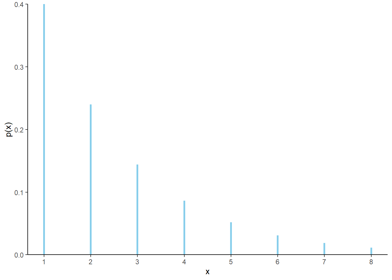
Figure 6.3: Impulse plot representing the Geometric(0.4) probability mass function.
Figure 6.4 displays a spinner corresponding to the Geometric(0.4) distribution. To simplify the display we have lumped \(x = 7, 8, 9, \ldots\) into one “7+” category.
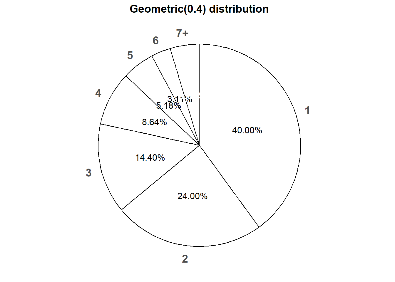
Figure 6.4: Spinner corresponding to the Geometric(0.4) distribution.
Below we see that simulation results are consistent with the theoretical results.
def count_until_first_success(omega):
    for i, w in enumerate(omega):
        if w == 1:
            return i + 1 # the +1 is for zero-based indexing

P = Bernoulli(0.4) ** inf

X = RV(P, count_until_first_success)
x = X.sim(10000)

x.plot()

Geometric(0.4).plot()
plt.show()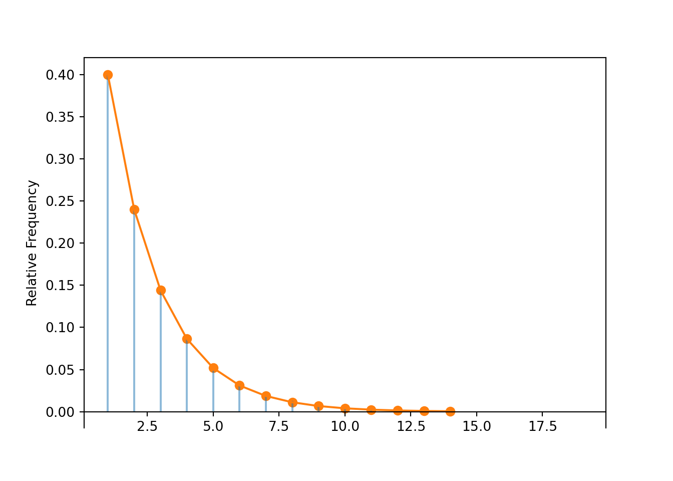
x.count_eq(3) / 10000, Geometric(0.4).pmf(3)## (0.1428, 0.144)
x.mean(), Geometric(0.4).mean()## (2.4842, 2.5)
x.var(), Geometric(0.4).var()## (3.58855036, 3.749999999999999)Definition 6.3 A discrete random variable \(X\) has a Geometric distribution with parameter \(p\in[0, 1]\) if its probability mass function is \[\begin{align*} p_{X}(x) & = p (1-p)^{x-1}, & x=1, 2, 3, \ldots \end{align*}\] If \(X\) has a Geometric(\(p\)) distribution \[\begin{align*} \textrm{E}(X) & = \frac{1}{p}\\ \textrm{Var}(X) & = \frac{1-p}{p^2} \end{align*}\]
plt.figure()

ps = [0.3, 0.5, 0.7, 0.9]

for p in ps:
  Geometric(p).plot()

plt.legend(ps)
plt.show()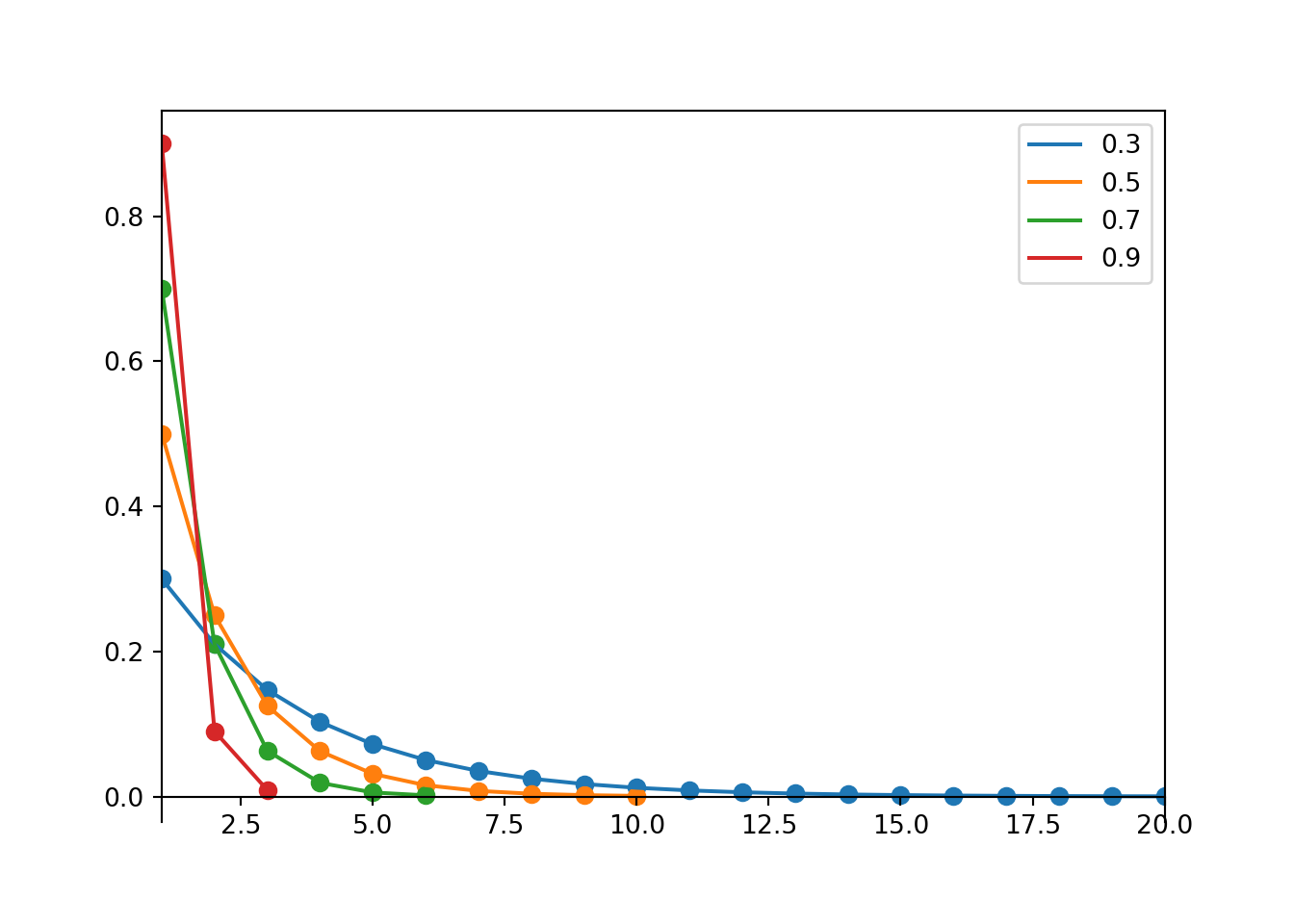
Suppose you perform Bernoulli(\(p\)) trials until a single success occurs and then stop. Let \(X\) be the total number of trials performed, including the success. Then \(X\) has a Geometric(\(p\)) distribution. In this situation, exactly \(x\) trials are performed if and only if - the first \(x-1\) trials are failures, and - the \(x\)th (last) trial results in success. Therefore \(\textrm{P}(X = x) = p(1-p)^{x-1}, x = 1, 2, 3, \ldots\).
Greater than \(x\) trials are needed to achieve the first success if and only if the first \(x\) trials result in failure. Therefore, \(\textrm{P}(X > x) = (1-p)^x, x = 1, 2, 3,\ldots\)
The fact that \(\textrm{E}(X)=1/p\) can be proven by conditioning on the result of the first trial and using the law of total expectation, similar to what we did in the first part of Example 5.46.
The variance of a Geometric distribution increases as \(p\) gets closer to 0. If \(p\) is close to 1, we expect to see success in the first few trials, but if \(p\) is close to 0, we could have to wait a larger number of trials until the first success occurs.
Example 6.11 Recall Example 3.5. You and your friend are playing the “lookaway challenge”. The game consists of possibly multiple rounds. In the first round, you point in one of four directions: up, down, left or right. At the exact same time, your friend also looks in one of those four directions. If your friend looks in the same direction you’re pointing, you win! Otherwise, you switch roles and the game continues to the next round — now your friend points in a direction and you try to look away. (So the player who starts as the pointer is the pointer in the odd-numbered rounds, and the player who starts as the looker is the pointer in the even-numbered rounds, until the game ends.) As long as no one wins, you keep switching off who points and who looks. The game ends, and the current “pointer” wins, whenever the “looker” looks in the same direction as the pointer. Let \(X\) be the number of rounds played in a game.
- Explain why \(X\) has a Geometric distribution, and specify the value of \(p\).
- Use the Geometric pmf (use software) to compute the probability that the player who starts as the pointer wins the game.
Solution. to Example 6.11
- \(X\) has a Geometric distribution with parameter \(p=0.25\).
- Each round is a trial,
- the round either results in success (current pointer wins the round and game ends) or failure (current pointer does not win the round and the game continues),
- the rounds are assumed to be independent
- the probability that the current point wins any particular round is 0.25
- and \(X\) counts the number of rounds until the first success
- The player who starts as the pointer wins the game if \(X\) is odd. So we need to sum the Geometric(0.25) pmf over \(x=1,3,5,\ldots\). See below.
Geometric pmfs are built in to Symbulate. We can find the probability that \(X\) is odd by summing the pmf over \(x = 1, 3, 5, \ldots\)
Geometric(0.25).pmf(range(1, 100, 2)).sum() # range(1, 100, 2) is odd numbers up to 100## 0.5714285714283882Below we simulate values of \(X\) in the lookaway challenge problem. The simulated distribution is consistent with the Geometric(0.4) distribution.
def count_rounds(sequence):
    for r, pair in enumerate(sequence):
        if pair[0] == pair[1]:
            return r + 1 # +1 for 0 indexing

P = BoxModel([1, 2, 3, 4], size = 2) ** inf

X = RV(P, count_rounds)

x = X.sim(25000)

x| Index | Result |
|---|---|
| 0 | 1 |
| 1 | 2 |
| 2 | 2 |
| 3 | 1 |
| 4 | 4 |
| 5 | 1 |
| 6 | 8 |
| 7 | 3 |
| 8 | 1 |
| ... | ... |
| 24999 | 8 |
Approximate distribution of the number of rounds.
x.plot()

Geometric(0.25).plot()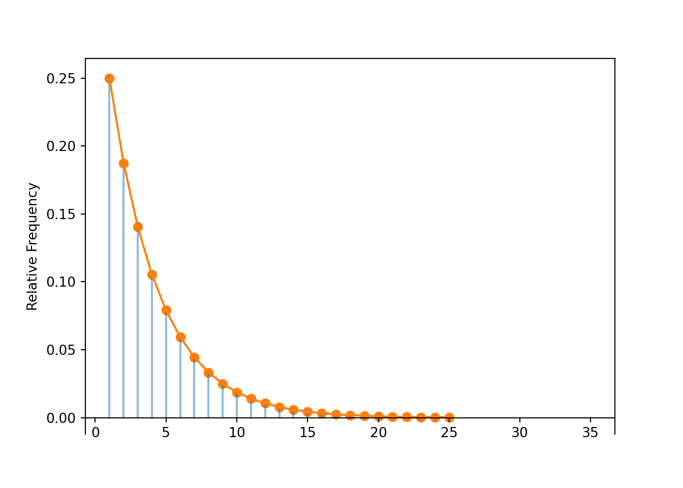
Approximate probability that the player who starts as the pointer wins the game (which occurs if the game ends in an odd number of rounds).
def is_odd(u):
    return (u % 2) == 1 # odd if the remainder when dividing by 2 is 1

x.count(is_odd) / x.count()
## 0.574046.3.2 Negative Binomial Distributions
Example 6.12 Maya is a basketball player who makes 86% of her free throw attempts. Suppose that she attempts free throws until she makes 5 and then stops. Let \(X\) be the total number of free throws she attempts. Assume shot attempts are independent.
- Does \(X\) have a Binomial distribution? Why or why not?
- What are the possible values of \(X\)? Is \(X\) discrete or continuous?
- Compute \(\textrm{P}(X=5)\)
- Compute \(\textrm{P}(X=6)\)
- Compute \(\textrm{P}(X=7)\)
- Compute \(\textrm{P}(Y=8)\)
- Find the probability mass function of \(X\).
- What seems like a reasonable general formula for \(\textrm{E}(X)\)? Interpret \(\textrm{E}(X)\) for this example.
- Would the variance be larger or smaller if attempted free throws until she made 10 instead of 5?
Solution. to Example 6.12
Show/hide solution
- \(X\) does not have a Binomial distribution since the number of trials is not fixed. The number of successes is fixed to be 5, but the number of trials is random.
- \(X\) can take values 5, 6, 7, \(\ldots\). Even though it is unlikely that \(X\) is very large, there is no fixed upper bound. Even though \(X\) can take infinitely values, \(X\) is a discrete random variables because it takes countably many possible values.
- In order for \(X\) to be 5, Maya must make her first 5 attempts. Since the attempts are independent \(\textrm{P}(X=5)=(0.86)^5=0.47\). If Maya does this every practice, then in about 47% of practices she will make her first five free throw attempts.
- In order for \(X\) to be 6, Maya must miss exactly one of her first 5 attempts and then make her 6th. (If she didn’t miss any of her first 5 attempts then she would be done in 5 attempts.) Consider the case where she misses her first attempt and then makes the next 5; this has probability \((1-0.86)(0.86)^5\). Any particular sequence with exactly 1 miss among the first 5 attempts and a make on the 6th attempt has this same probability. There are 5 “spots” for where the 1 miss can go, so there are \(\binom{5}{1} = 5\) possible sequences. Therefore \[ \textrm{P}(X=6) = \binom{5}{1}(0.86)^5(1-0.86)^1 = 0.329 \] Equivalently, the 4 successes, excluding the final success, must occur in the first 5 attempts, so there are \(\binom{5}{4}\) possible sequences. Note that \(\binom{5}{1} = 5 = \binom{5}{4}\). So we can also write \[ \textrm{P}(X=6) = \binom{5}{4}(0.86)^5(1-0.86)^1 = 0.329 \]
- In order for \(X\) to be 7, Maya must miss exactly two of her first 6 attempts and then make her 7th. Any particular sequence of this form has probability \((0.86)^5(1-0.86)^2\) and there are \(\binom{6}{2}=\binom{6}{4}\) possible sequences. Therefore \[\begin{align*} \textrm{P}(X=7) & = \binom{6}{2}(0.86)^5(1-0.86)^2 = 0.138\\ & = \binom{6}{4}(0.86)^5(1-0.86)^2 \end{align*}\]
- In order for \(X\) to be 8, Maya must miss exactly three of her first 7 attempts and then make her 8th. Any particular sequence of this form has probability \((0.86)^5(1-0.86)^3\) and there are \(\binom{7}{3}=\binom{7}{4}\) possible sequences. Therefore \[\begin{align*} \textrm{P}(X=8) & = \binom{7}{3}(0.86)^5(1-0.86)^3 = 0.045\\ & = \binom{7}{4}(0.86)^5(1-0.86)^3 \end{align*}\]
- In order for \(X\) to take value \(x\), the last trial must be success and the first \(x-1\) trials must consist of \(5-1=4\) successes and \(x-5\) failures. There are \(\binom{x-1}{5-1}\) ways to have \(4\) successes among the first \(x-1\) trials. (This is the same as saying there are \(\binom{x-1}{x-5}\) ways to have \(x-5\) failures among the first \(x-1\) trials.) \[\begin{align*} p_X(x) = \textrm{P}(X=x) & = \binom{x-1}{5-1}(0.86)^5(1-0.86)^{x-5}, \qquad x = 5, 6, 7, \ldots\\ & = \binom{x-1}{x-5}(0.86)^5(1-0.86)^{x-5}, \qquad x = 5, 6, 7, \ldots \end{align*}\]
- On average it takes \(1/0.86 = 1.163\) attempts to make a free throw, so it seems reasonable that it would take on average \(5(1/0.86)=5.81\) attempts to make 5 free throws. If Maya does this at every practice, it takes her on average 5.8 attempts to make 5 free throws.
- The variance would be larger with 10 attempts.
r = 5
def count_until_rth_success(omega):
    trials_so_far = []
    for i, w in enumerate(omega):
        trials_so_far.append(w)
        if sum(trials_so_far) == r:
            return i + 1

P = Bernoulli(0.86) ** inf

X = RV(P, count_until_rth_success)
x = X.sim(10000)

x.plot()

NegativeBinomial(r = 5, p = 0.86).plot()
plt.show()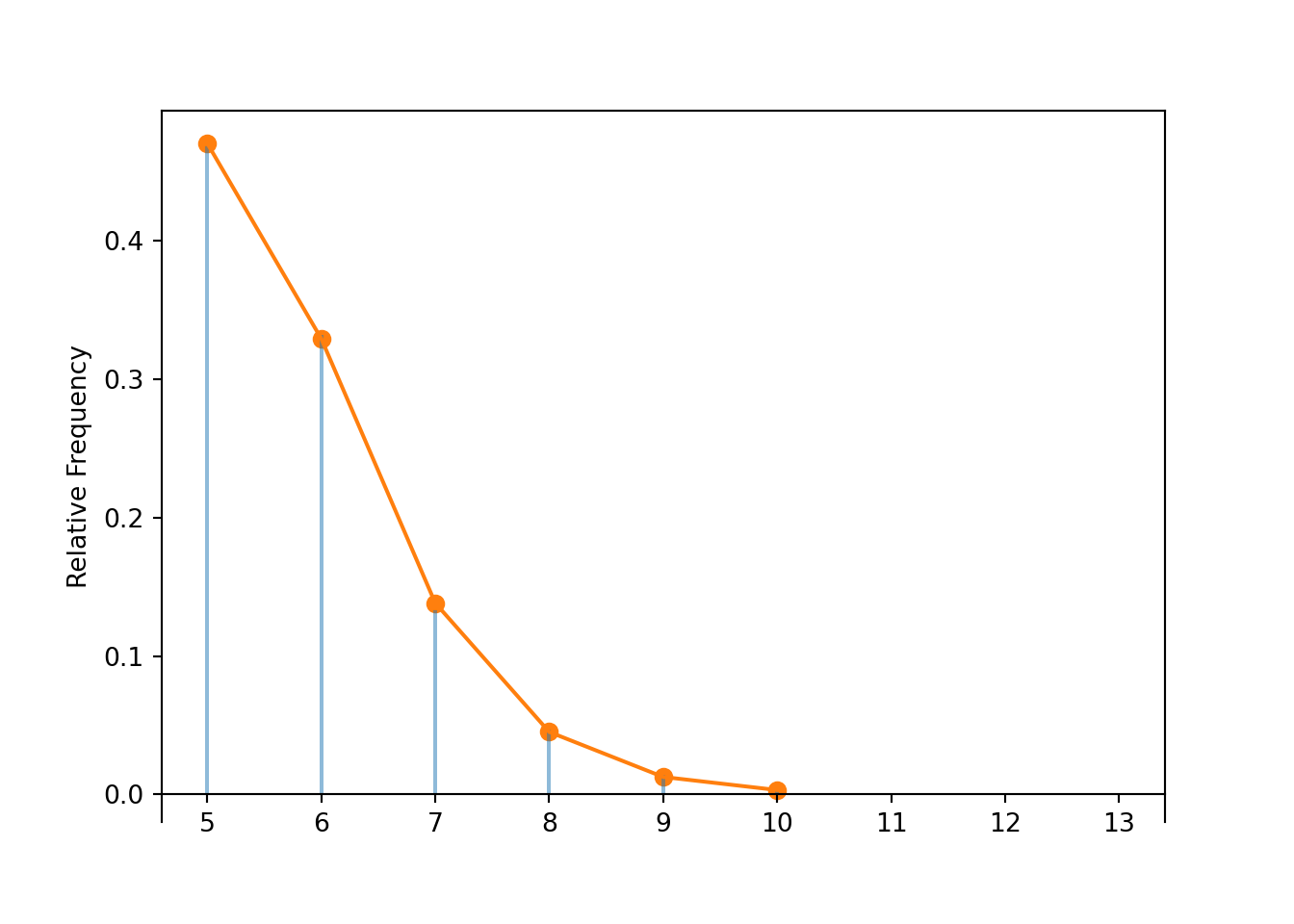
x.count_eq(7) / 10000, NegativeBinomial(r = 5, p = 0.86).pmf(7)## (0.1334, 0.1383055431744)
x.mean(), NegativeBinomial(r = 5, p = 0.86).mean()## (5.8221, 5.813953488372094)
x.var(), NegativeBinomial(r = 5, p = 0.86).var()## (0.9790515900000002, 0.9464575446187132)Definition 6.4 A discrete random variable \(X\) has a Negative Binomial distribution with parameters \(r\), a positive integer, and \(p\in[0, 1]\) if its probability mass function is \[\begin{align*} p_{X}(x) & = \binom{x-1}{r-1}p^r(1-p)^{x-r}, & x=r, r+1, r+2, \ldots \end{align*}\] If \(X\) has a NegativeBinomial(\(r\), \(p\)) distribution \[\begin{align*} \textrm{E}(X) & = \frac{r}{p}\\ \textrm{Var}(X) & = \frac{r(1-p)}{p^2} \end{align*}\]
Suppose you perform a sequence of Bernoulli(\(p\)) trials until \(r\) successes occur and then stop. Let \(X\) be the total number of trials performed, including the trials on which the successes occur. Then \(X\) has a NegativeBinomial(\(r\),\(p\)) distribution. In this situation, exactly \(x\) trials are performed if and only if
- there are exactly \(r-1\) successes among the first \(x-1\) trials, and
- the \(x\)th (last) trial results in success.
There are \(\binom{x-1}{r-1}\) possible sequences that satisfy the above, and each of these sequences — with \(r\) successes and \(x-r\) failures — has probability \(p^r(1-p)^{x-r}\).
Example 6.13 What is another name for a NegativeBinomial(1,\(p\)) distribution?
Solution. to Example 6.13
Show/hide solution
A NegativeBinomial(1,\(p\)) distribution is a Geometric(\(p\)) distribution.
Example 6.14 Suppose \(X_1, \ldots, X_r\) are independent each with a Geometric(\(p\)) distribution. What is the distribution of \(X_1+\cdots + X_r\)? Find the expected value and variance of this distribution.
Solution. to Example 6.14
Show/hide solution
Consider a long sequence of Bernoulli(\(p\)) trials. Let \(X_1\) count the number of trials until the 1st success occurs. Starting immediately after the first success occurs, let \(X_2\) count the number of additional trials until the 2nd success occurs, so that \(X_1+X_2\) is the total number of trials until the first 2 successes occur. Since \(X_1\) and \(X_2\) are independent, then the two sets of trials are independent. That is, \(X_1+X_2\) counts the number of trials until 2 successes occur in Bernoulli(\(p\)) trials, so \(X_1+X_2\) has a Negative Binomial(2, \(p\)) distribution. Continuining in this way we see that if \(X_1, \ldots, X_r\) are independent each with a Geometric(\(p\)) distribution then \((X_1+\cdots+X_r)\) has a NegativeBinomial(\(r\),\(p\)) distribution.
If \(X\) has a NegativeBinomial(\(r\),\(p\)) distribution then it has the same distributional properties as \((X_1+\cdots+X_r)\) where \(X_1, \ldots, X_r\) are independent each with a Geometric(\(p\)) distribution. Therefore we can compute the mean of a Negative Binomial distribution by computing \[ \textrm{E}(X_1+\cdots+X_r) =\textrm{E}(X_1)+\cdots+\textrm{E}(X_r) = \frac{1}{p} + \cdots + \frac{1}{p} = \frac{r}{p} \] We can use a similar technique to compute the variance of a Negative Binomial distribution, because the \(X_i\)s are independent. \[ \textrm{Var}(X_1+\cdots+X_r) \stackrel{\text{(independent)}}{=}\textrm{Var}(X_1)+\cdots+\textrm{Var}(X_r) = \frac{1-p}{p^2} + \cdots + \frac{1-p}{p^2} = \frac{r(1-p)}{p^2} \]
6.3.3 Pascal distributions
In a Negative Binomial situation, the total number of successes is fixed (\(r\)), i.e., not random. What is random is the number of failures, and hence the total number of trials.
Our definition of a Negative Binomial distribution (and hence a Geometric distribution) provides a model for a random variable which counts the number of Bernoulli(\(p\)) trials required until \(r\) successes occur, including the \(r\) trials on which success occurs, so the possible values are \(r, r+1, r+2,\ldots\)
There is an alternative definition of a Negative Binomial distribution (and hence a Geometric distribution) which provides a model for a random variable which counts the number of failures in Bernoulli(\(p\)) trials required until \(r\) successes occur, excluding the \(r\) trials on which success occurs, so the possible values are \(0, 1, 2, \ldots\) Many software programs, including R, use this alternative definition. In Symbulate, a Pascal(\(r\), \(p\)) distribution follows this alternate definition. In Symbulate,
- The possible values of a NegativeBinomial(\(r\), \(p\)) distribution are \(r, r+1, r+2,\ldots\)
- The possible values of a Pascal(\(r\), \(p\)) distribution are \(0, 1, 2,\ldots\)
If \(X\) has a NegativeBinomial(\(r\), \(p\)) distribution then \((X-r)\) has a Pascal(\(r\), \(p\)) distribution.