4.7 Joint distributions
Most interesting problems involve two or more117 random variables defined on the same probability space. In these situations, we can consider how the variables vary together, or jointly, and study their relationship. The joint distribution of random variables \(X\) and \(Y\) (defined on the same probability space) is a probability distribution on \((x, y)\) pairs. In this context, the distribution of one of the variables alone is called a marginal distribution.
Think of a joint distribution of two random variables as being represented by a spinner or “globe” that returns pairs of values.
4.7.1 Joint probability mass functions
The joint distribution of table discrete random variables can be summarized in a table of possible pairs and their probabilities.
Example 4.31 Flip a fair coin four times and record the results in order, e.g. HHTT means two heads followed by two tails. Recall that in Section 1.6 we considered the proportion of the flips which immediately follow a H that result in H. We cannot measure this proportion if no flips follow a H, i.e. the outcome is either TTTT or TTTH; in these cases, we would discard the outcome and try again.
Let:
- \(Z\) be the number of flips immediately following H.
- \(Y\) be the number of flips immediately following H that result in H.
- \(X = Y/Z\) be the proportion of flips immediately following H that result in H.
- Make a table of all possible outcomes and the corresponding values of \(Z, Y, X\).
- Make a two-way table representing the joint probability mass function of \(Y\) and \(Z\).
- Construct a spinner for simulating \((Y, Z)\) pairs.
- Make a table specifying the pmf of \(X\).
Solution. to Example 4.31
Show/hide solution
- See Table 4.4. The flips which follow H are in bold.
- See Table 4.5. There are 16 possible four flip sequences but two of these — TTTH and TTTT — are discarded. So there are only 14 possible outcomes of interest, all equally likely. We can find the possible \((Y, Z)\) pairs and their probabilities from Table 4.4. For example, \(p_{Y,Z}(1,2) = \textrm{P}(Y=1, Z=2) = \textrm{P}(\{HHTH, HTHH, HHTT, THHT\})=4/14\); \(p_{Y,Z}(2,3) = \textrm{P}(Y=2, Z=3) = \textrm{P}(\{HHHT\})=1/14\).
- See Figure 4.24. The spinner returns possible \((Y, Z)\) pairs according to their joint probabilities.
- See Table 4.6. We started with the table of possible values, but if we hadn’t we still could have obtained the marginal distribution of \(X = Y / Z\) from from the joint distribution of \((Y, Z)\). For example \(p_X(1) = \textrm{P}(X = 1) = \textrm{P}(Y = 1, Z = 1) + \textrm{P}(Y = 2, Z = 2) + \textrm{P}(Y = 3, Z = 3) = 3/14\).
| Outcome | \(Z\) | \(Y\) | \(X = Y/Z\) |
|---|---|---|---|
| HHHH | 3 | 3 | 1 |
| HHHT | 3 | 2 | 2/3 |
| HHTH | 2 | 1 | 1/2 |
| HTHH | 2 | 1 | 1/2 |
| THHH | 2 | 2 | 1 |
| HHTT | 2 | 1 | 1/2 |
| HTHT | 2 | 0 | 0 |
| HTTH | 1 | 0 | 0 |
| THHT | 2 | 1 | 1/2 |
| THTH | 1 | 0 | 0 |
| TTHH | 1 | 1 | 1 |
| HTTT | 1 | 0 | 0 |
| THTT | 1 | 0 | 0 |
| TTHT | 1 | 0 | 0 |
| TTTH | 0 | not defined | not defined |
| TTTT | 0 | not defined | not defined |
| \(y, z\) | 1 | 2 | 3 |
|---|---|---|---|
| 0 | 5/14 | 1/14 | 0 |
| 1 | 1/14 | 4/14 | 0 |
| 2 | 0 | 1/14 | 1/14 |
| 3 | 0 | 0 | 1/14 |
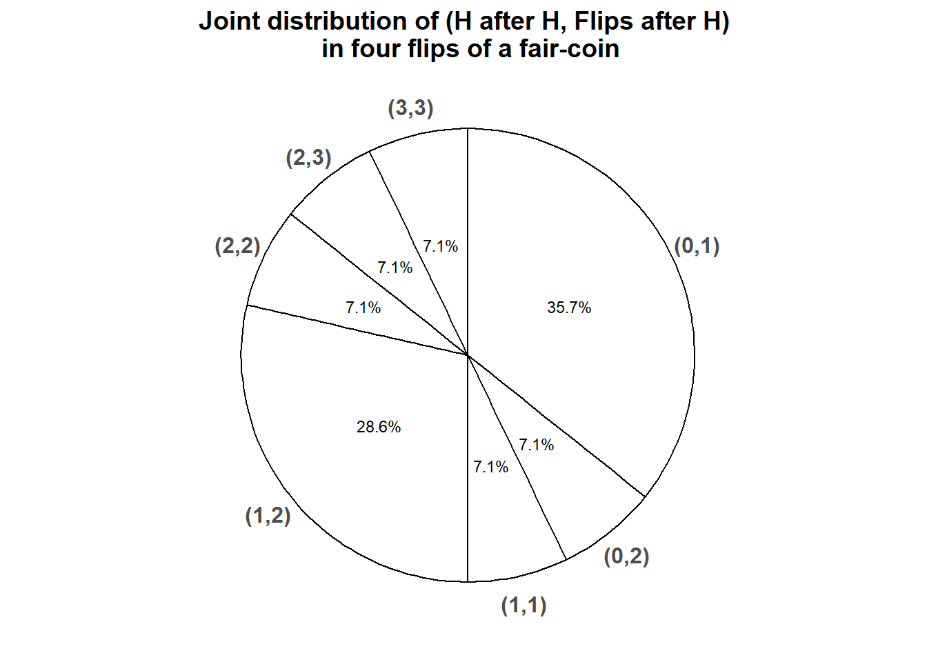
Figure 4.24: Spinner representing the joint probability mass function of \((Y, Z)\) where \(Z\) is the number of flips immediately following H, and \(Y\) is the number of flips immediately following H that result in H, for four flips of a fair coin.
| \(x\) | \(p_X(x)\) |
|---|---|
| 0 | 6/14 |
| 1/2 | 4/14 |
| 2/3 | 1/14 |
| 1 | 3/14 |
Definition 4.9 The joint probability mass function (pmf) of two discrete random variables \((X,Y)\) defined on a probability space with probability measure \(\textrm{P}\) is the function \(p_{X,Y}:\mathbb{R}^2\mapsto[0,1]\) defined by \[ p_{X,Y}(x,y) = \textrm{P}(X= x, Y= y) \qquad \text{ for all } x,y \]
The axioms of probability imply that a valid joint pmf must satisfy
\[\begin{align*} p_{X,Y}(x,y) & \ge 0 \quad \text{for all $x, y$}\\ p_{X,Y}(x,y) & >0 \quad \text{for at most countably many $(x,y)$ pairs (the possible values, i.e., support)}\\ \sum_x \sum_y p_{X,Y}(x,y) & = 1 \end{align*}\]Remember to specify the possible \((x, y)\) pairs when defining a joint pmf.
For example, let \(X\) be the sum and \(Y\) the larger of two rolls of a fair four-sided die. The the joint pmf of \(X\) and \(Y\) is represented in Table 2.14. We can express the table a little more compactly as \[ p_{X, Y}(x, y) = \begin{cases} 2/16, & y = 2, 3, 4, \qquad x = y+1, \ldots, 2y-1\\ 1/16, & y = 1, 2, 3, 4, \quad x = 2y\\ 0, & \text{otherwise} \end{cases} \] Notice the specification of the possible \((x, y)\) pairs.
Example 4.32 Let \(X\) be the number of home runs hit by the home team, and \(Y\) the number of home runs hit by the away team in a randomly selected Major League Baseball game. Suppose that \(X\) and \(Y\) have joint pmf
\[ p_{X, Y}(x, y) = \begin{cases} e^{-2.3}\frac{1.2^{x}1.1^{y}}{x!y!}, & x = 0, 1, 2, \ldots; y = 0, 1, 2, \ldots,\\ 0, & \text{otherwise.} \end{cases} \]
- Compute and interpret the probability that the home teams hits 2 home runs and the away team hits 1 home run.
- Construct a two-way table representation of the joint pmf.
- Compute and interpret the probability that each team hits at most 4 home runs.
- Compute and interpret the probability that both teams combine to hit a total of 3 home runs.
- Compute and interpret the probability that the home team and the away team hit the same number of home runs.
Solution. to Example 4.32
Show/hide solution
- Plug \(x=2, y=1\) into the joint pmf: \(\textrm{P}(X = 2, Y = 1) = p_{X, Y}(2, 1) = e^{-2.3}\frac{1.2^2 1.1^1}{2!1!}= 0.0794\). Over many games, the home teams hits 2 home runs and the away team hits 1 home run in about 7.9% of games.
- See Table 4.7 and Figure 4.25 below. The possible values of \(x\) are 0, 1, 2, \(\ldots\), and similarly for \(y\), and any \((x, y)\) pair of these values is possible. Plug each \((x, y)\) pair into \(p_{X,Y}\) like in the previous part.
- Sum the joint pmf over the top left corner of the table representing the 25 \((x, y)\) pairs where both coordinates are at most 4: (0, 0), (0, 1), (0, 2), (0, 3), (0, 4), (1, 0), \(\ldots\), (4, 4). There is no easy way to do it other than adding all the numbers. \[\begin{align*} \textrm{P}(X \le 4, Y \le 4) & = p_{X, Y}(0, 0) + p_{X, Y}(0, 1)+p_{X, Y}(0, 2)+p_{X, Y}(0, 3)+p_{X, Y}(0, 4) + p_{X, Y}(1, 0)\cdots+p_{X, Y}(4, 4)\\ & = 0.100 + 0.110 + 0.061 + 0.022 + 0.006 + \cdots + 0.0005 = 0.987 \end{align*}\] While technically any pair of nonnegative integers is possible, almost all of the probability is concentrated on pairs where neither coordinate is more than 4. Over many games, neither team hits more than 4 home runs in 98.7% of games.
- The corresponding \((x, y)\) pairs are (0, 3), (1, 2), (2, 1), (3, 0). \[\begin{align*} \textrm{P}(X + Y = 3) & = p_{X, Y}(0, 3) + p_{X, Y}(1, 2)+p_{X, Y}(2, 1)+p_{X, Y}(3, 0)\\ & = 0.022 + 0.073 + 0.079 + 0.029 = 0.203 \end{align*}\] We will see an easier way to do this later. Over many games, both teams combine to hit a total of 3 home runs in about 20.3% of games.
- Sum over values where \(x=y\), the diagonal cells of the table. \[\begin{align*} \textrm{P}(X = Y) & = p_{X, Y}(0, 0) + p_{X, Y}(1, 1) + p_{X, Y}(2, 2) + \cdots \\ & = 0.100 + 0.132 + 0.044 + \cdots = 0.283. \end{align*}\] Over many games, the two teams hit in the same number of home runs in about 28.3% of games. Technically this is an infinite series, but the contributions of the terms after (6, 6) are negligible. The sum can be written as an infinite series, but there isn’t a shortcut to evaluate it. \[ \textrm{P}(X = Y) = \sum_{u = 0}^\infty e^{-2.3}\frac{1.2^u 1.1^u}{u!u!} = 0.283. \]
| x, y | 0 | 1 | 2 | 3 | 4 | 5 | 6 | 7 | 8 | … | Total |
|---|---|---|---|---|---|---|---|---|---|---|---|
| 0 | 0.10026 | 0.11028 | 0.06066 | 0.02224 | 0.00612 | 0.00135 | 0.00025 | 0.00004 | 0.00001 | 0.30119 | |
| 1 | 0.12031 | 0.13234 | 0.07279 | 0.02669 | 0.00734 | 0.00161 | 0.00030 | 0.00005 | 0.00001 | 0.36143 | |
| 2 | 0.07219 | 0.07941 | 0.04367 | 0.01601 | 0.00440 | 0.00097 | 0.00018 | 0.00003 | 0.00000 | 0.21686 | |
| 3 | 0.02887 | 0.03176 | 0.01747 | 0.00641 | 0.00176 | 0.00039 | 0.00007 | 0.00001 | 0.00000 | 0.08674 | |
| 4 | 0.00866 | 0.00953 | 0.00524 | 0.00192 | 0.00053 | 0.00012 | 0.00002 | 0.00000 | 0.00000 | 0.02602 | |
| 5 | 0.00208 | 0.00229 | 0.00126 | 0.00046 | 0.00013 | 0.00003 | 0.00001 | 0.00000 | 0.00000 | 0.00625 | |
| 6 | 0.00042 | 0.00046 | 0.00025 | 0.00009 | 0.00003 | 0.00001 | 0.00000 | 0.00000 | 0.00000 | 0.00125 | |
| 7 | 0.00007 | 0.00008 | 0.00004 | 0.00002 | 0.00000 | 0.00000 | 0.00000 | 0.00000 | 0.00000 | 0.00021 | |
| 8 | 0.00001 | 0.00001 | 0.00001 | 0.00000 | 0.00000 | 0.00000 | 0.00000 | 0.00000 | 0.00000 | 0.00003 | |
| … | |||||||||||
| Total | 0.33287 | 0.36616 | 0.20139 | 0.07384 | 0.02031 | 0.00447 | 0.00082 | 0.00013 | 0.00002 | 1.00000 |
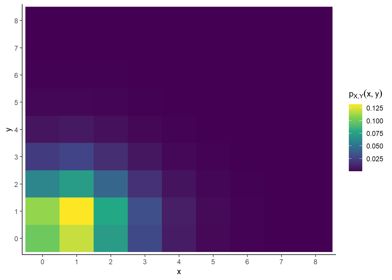
Figure 4.25: Tile plot representing the joint distribution of \(X\) and \(Y\) in Example 4.32.
Recall that we can obtain marginal distributions from a joint distribution. Marginal pmfs are determined by the joint pmf via the law of total probability. If we imagine a plot with blocks whose heights represent the joint probabilities, the marginal probability of a particular value of one variable can be obtained by “stacking” all the blocks corresponding to that value. In terms of a two-way table, a marginal distribution can be obtained by “collapsing” the table by summing rows or columns.
\[\begin{align*} p_X(x) & = \sum_y p_{X,Y}(x,y) & & \text{a function of $x$ only} \\ p_Y(y) & = \sum_x p_{X,Y}(x,y) & & \text{a function of $y$ only} \\ \end{align*}\]Example 4.33 Continuining Example 4.32. Let \(X\) be the number of home runs hit by the home team, and \(Y\) the number of home runs hit by the away team in a randomly selected Major League Baseball game. Suppose that \(X\) and \(Y\) have joint pmf
\[ p_{X, Y}(x, y) = \begin{cases} e^{-2.3}\frac{1.2^{x}1.1^{y}}{x!y!}, & x = 0, 1, 2, \ldots; y = 0, 1, 2, \ldots,\\ 0, & \text{otherwise.} \end{cases} \]
- Compute and interpret the probability that the home team hits 2 home runs.
- Find the marginal pmf of \(X\), and identify the marginal distribution by name.
- Compute and interpret the probability that the away team hits 1 home run.
- Find the marginal pmf of \(Y\), and identify the marginal by name.
- Use the joint pmf to compute the probability that the home team hits 2 home runs and the away team hits 1 home run. How does it relate to the marginal probabilities from the previous parts? What does this imply about the events \(\{X = 2\}\) and \(\{Y = 1\}\)?
- How does the joint pmf relate to the marginal probabilities from the previous parts? What do you think this implies about \(X\) and \(Y\)?
- In light of the previous part, how you could use spinners to simulate and \((X, Y)\) pair?
Solution. to Example 4.33
Show/hide solution
- Sum over the values of \(y\) in the \(x=2\) row of the joint pmf table. Mathematically, we plug 2 in for \(x\) in the joint pmf and sum over all the possible values of \(y\) \[\begin{align*} \textrm{P}(X = 2) & = \sum_{y=0}^\infty p_{X, Y}(2, y)\\ & = \sum_{y=0}^\infty e^{-2.3}\frac{1.2^2 1.1^y}{2!y!}\\ & = e^{-2.3}\frac{1.2^2}{2!}\sum_{y=0}^\infty \frac{1.1^y}{y!}\\ & = e^{-2.3}\frac{1.2^2}{2!}\left(e^{1.1}\right)\\ & = e^{-1.2}\frac{1.2^2}{2!} = 0.217. \end{align*}\] Over many games, the home team hits 2 home runs in about 21.7% of games.
- The possible values of \(X\) are \(0, 1, 2, \ldots\). For corresponding probabilities see the total column containing the row sums in Table 4.7. Mathematically, for a given \(x\) (like 2 in the previous part) we plug it into the joint pmf and sum over the possible \(y\) values. Basically, we repeat the calculation from the previous part but for a generic possible value of \(x= 0, 1, 2\ldots\) \[\begin{align*} p_X(x) & = \sum_{y=0}^\infty p_{X, Y}(x, y)\\ & = \sum_{y=0}^\infty e^{-2.3}\frac{1.2^x 1.1^y}{x!y!}\\ & = e^{-2.3}\frac{1.2^x}{x!}\sum_{y=0}^\infty \frac{1.1^y}{y!}\\ & = e^{-2.3}\frac{1.2^x}{x!}\left(e^{1.1}\right)\\ & = e^{-1.2}\frac{1.2^x}{x!}. \end{align*}\] The marginal distribution of \(X\) is the Poisson(1.2) distribution. Notice that the marginal pmf of \(X\) is a function of values of \(X\) alone: \(p_X(x)= e^{-1.2}\frac{1.2^x}{x!}, x = 0, 1, 2\ldots\).
- Sum over the values of \(x\) in the \(y=1\) column of the joint pmf table. Mathematically, we plug 1 in for \(y\) in the joint pmf and sum over all the possible values of \(x\) \[\begin{align*} \textrm{P}(Y = 1) & = \sum_{x=0}^\infty p_{X, Y}(x, 1)\\ & = \sum_{x=0}^\infty e^{-2.3}\frac{1.2^x 1.1^1}{x!1!}\\ & = e^{-2.3}\frac{1.1^1}{1!}\sum_{x=0}^\infty \frac{1.2^x}{x!}\\ & = e^{-2.3}\frac{1.1^1}{1!}\left(e^{1.2}\right)\\ & = e^{-1.1}\frac{1.1^1}{1!} = 0.366. \end{align*}\] Over many games, the away team hits 1 home run in about 36.6% of games.
- The possible values of \(Y\) are \(0, 1, 2, \ldots\). For corresponding probabilities see the total row containing the column sums in Table 4.7. Mathematically, for a given \(y\) (like 1 in the previous part) we plug it into the joint pmf and sum over the possible \(x\) values. Basically, we repeat the calculation from the previous part but for a generic possible value of \(y= 0, 1, 2\ldots\) \[\begin{align*} \textrm{P}(Y = y)& = \sum_{x=0}^\infty p_{X, Y}(x, y)\\ & = \sum_{x=0}^\infty e^{-2.3}\frac{1.2^x 1.1^y}{x!y!}\\ & = e^{-2.3}\frac{1.1^y}{y!}\sum_{x=0}^\infty \frac{1.2^x}{x!}\\ & = e^{-2.3}\frac{1.1^y}{y!}\left(e^{1.2}\right)\\ & = e^{-1.1}\frac{1.1^y}{y!}. \end{align*}\] The marginal distribution of \(Y\) is the Poisson(1.1) distribution. Notice that the marginal pmf of \(Y\) is a function of values of \(Y\) alone: \(p_Y(y)= e^{-1.1}\frac{1.1^y}{y!}, y = 0, 1, 2\ldots\).
- The joint probability turns out to be the product of the marginal probabilities we computed earlier in this example. \[ \scriptsize{ \textrm{P}(X = 2, Y=1) = p_{X,Y}(2, 1) = 0.079= e^{-2.3}\frac{1.2^{2}1.1^{1}}{2!1!} = \left(e^{-1.2}\frac{1.2^{2}}{2!}\right)\left(e^{-1.1}\frac{1.1^{1}}{1!}\right) = (0.217)(0.366) = p_X(2)p_Y(1) = \textrm{P}(X = 2)\textrm{P}(Y = 1)} \] Therefore, the \(\{X = 2\}\) and \(\{Y = 1\}\) are independent events.
- Similar to the previous part, we see that the joint pmf factors into the product of the marginal pmfs we identified earlier in this example. \[ \scriptsize{ \textrm{P}(X = x, Y=y) = p_{X,Y}(x, y) = e^{-2.3}\frac{1.2^{x}1.1^{y}}{x!y!} = \left(e^{-1.2}\frac{1.2^{x}}{x!}\right)\left(e^{-1.1}\frac{1.1^{y}}{y!}\right) = p_X(x)p_Y(y) = \textrm{P}(X = x)\textrm{P}(Y = y)} \] Recalling the general relationship “independent if and only if joint equals product of marginals” this seems to imply \(X\) and \(Y\) are independent random variables.
- We could construct a spinner corresponding to the joint distribution that returns \((X, Y)\) pairs. But since \(X\) and \(Y\) are independent we can spin a Poisson(1.2) distribution spinner to simulate \(X\), and spin a Poisson(1.1) distribution spinner to simulate \(Y\). That is, since \(X\) and \(Y\) are independent we can simulate their values separately.
In the previous example, the marginal distribution of \(X\) is the Poisson(1.2) distribution and the marginal distribution of \(Y\) is the Poisson(1.1) distribution. Furthermore \(X\) and \(Y\) are also independent, because their marginal pmf is the product of their joint pmfs. We will study independence of random variables in more detail soon.
The code below simulates \((X, Y)\) pairs from the joint distribution in Example 4.32; compare the results to Table 4.7 and Figure 4.25 The * syntax indicates that \(X\) and \(Y\) are independent.
The code X, Y = RV(Poisson(1.2) * Poisson(1.1)) defines the joint distribution of \(X\) and \(Y\) by specifying
- The marginal distribution of \(X\) is Poisson(1.2)
- The marginal distribution of \(Y\) is Poisson(1.1)
- The joint distribution of \(X\) and \(Y\) is the product (
*) of the marginal distributions, so \(X\) and \(Y\) are independent.
X, Y = RV(Poisson(1.2) * Poisson(1.1))

x_and_y = (X & Y).sim(10000)

x_and_y| Index | Result |
|---|---|
| 0 | (1, 1) |
| 1 | (1, 1) |
| 2 | (0, 2) |
| 3 | (0, 0) |
| 4 | (2, 2) |
| 5 | (2, 1) |
| 6 | (1, 0) |
| 7 | (1, 0) |
| 8 | (1, 0) |
| ... | ... |
| 9999 | (2, 2) |
x_and_y.tabulate(normalize = True)| Value | Relative Frequency |
|---|---|
| (0, 0) | 0.1008 |
| (0, 1) | 0.1159 |
| (0, 2) | 0.0567 |
| (0, 3) | 0.0225 |
| (0, 4) | 0.0068 |
| (0, 5) | 0.0019 |
| (0, 6) | 0.0001 |
| (1, 0) | 0.1197 |
| (1, 1) | 0.13 |
| (1, 2) | 0.0733 |
| (1, 3) | 0.0258 |
| (1, 4) | 0.0079 |
| (1, 5) | 0.0012 |
| (1, 6) | 0.0004 |
| (2, 0) | 0.0718 |
| (2, 1) | 0.0835 |
| (2, 2) | 0.042 |
| (2, 3) | 0.0166 |
| (2, 4) | 0.0055 |
| ... | ... |
| (7, 2) | 0.0001 |
| Total | 0.9999999999999994 |
x_and_y.plot('tile')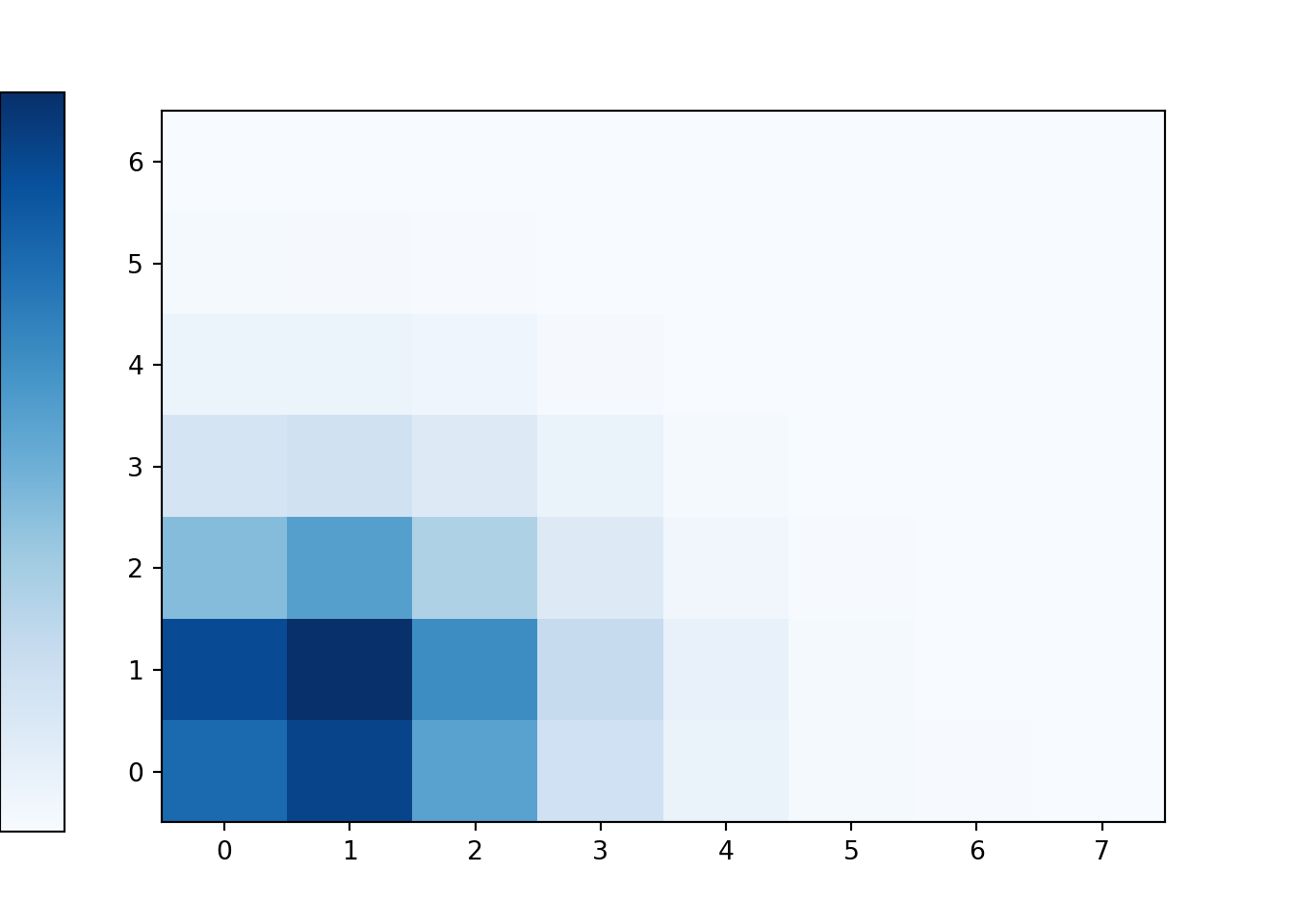
Figure 4.26: Tile plot of \((X, Y)\) pairs simulated from the joint distribution in Example 4.32.
Example 4.34 (Blitzstein’s chicken and egg story.) Suppose \(N\), the number of eggs a chicken lays in a randomly selected week, has a Poisson(\(6.5\)) distribution. Each egg hatches with probability \(0.8\), independently of all other eggs. Let \(X\) be the number of eggs that hatch. Let \(p_{N, X}\) denote the joint pmf of \(N\) and \(X\).
- Identify the possible \((N, X)\) pairs.
- Identify the conditional distribution of \(X\) given \(N=7\).
- Compute and interpret \(p_{N, X}(7, 7)\). Hint: compute \(\textrm{P}(X = 7|N = 7)\) and use the multiplication rule.
- Compute and interpret \(p_{N, X}(7, 5)\)
- Identify the conditional distribution of \(X\) given \(N=n\) for a generic \(n=0, 1, 2, \ldots\).
- Find an expression for the joint pmf \(p_{N, X}\). Be sure to specify the possible values.
- Are \(N\) and \(X\) independent?
- Make a table of the joint pmf.
Solution. to Example 4.34
Show/hide solution
- Since \(N\) has a Poisson distribution its possible values are \(0, 1, 2, \ldots\). \(X\) also takes nonnegative integer values, but since the number of eggs that hatch can’t be more than the number of eggs, we must have \(X \le N\). So the possible \((n, x)\) pairs satisfy \[ n = 0, 1, 2, \ldots; x = 0, 1, \ldots, n \]
- Given \(N=7\) eggs, each of the 7 eggs either hatches or not, with probability 0.8, independently, and \(X\) counts the number of eggs that hatch. This is a Binomial situation with 7 independent trials and probability of success 0.8 on each trial. Therefore the conditional distribution of \(X\) given \(N=7\) is the Binomial(7, 0.8) distribution.
- Given that there are 7 eggs, the probability that they all hatch (independently) is \(\textrm{P}(X = 7|N = 7) = 0.8^7\). \[\begin{align*} p_{N, X}(7, 7) & = \textrm{P}(N = 7, X = 7) & & \\ & = \textrm{P}(X = 7 | N = 7)\textrm{P}(N = 7) & & \text{multiplication rule}\\ & = 0.8^7\textrm{P}(N=7) & & \text{conditional Binomial}\\ & = 0.8^7\left(e^{-6.5}\frac{6.5^7}{7!}\right) & & \text{marginal Poisson}\\ & = e^{-6.5}\frac{(0.8\times 6.5)^7}{7!} = 0.030 & & \end{align*}\] In about 3% of weeks the chicken lays 7 eggs and all 7 hatch.
- Given that there are 7 eggs, the probability that exactly 5 hatch (independently) is \(\textrm{P}(X = 5|N = 7) = \binom{7}{5}(0.8)^5(1-0.8)^{7-5}\), since the conditional distribution of \(X\) given \(N=7\) is the Binomial(7, 0.8) distribution. \[\begin{align*} p_{N, X}(7, 5) & = \textrm{P}(N = 7, X = 5) & & \\ & = \textrm{P}(X = 5 | N = 7)\textrm{P}(N = 7) & & \text{multiplication rule}\\ & = \left(\binom{7}{5}(0.8)^5(1-0.8)^{7-5}\right)\textrm{P}(N=7) & & \text{conditional Binomial}\\ & = \left(\binom{7}{5}(0.8)^5(1-0.8)^{7-5}\right)\left(e^{-6.5}\frac{6.5^7}{7!}\right) & & \text{marginal Poisson}\\ & = e^{-6.5}\left(\frac{(0.8\times 6.5)^5}{5!}\right)\left(\frac{((1-0.8)\times 6.5)^{7-5}}{(7-5)!}\right) = 0.040 & & \text{algebra with binomial coefficient} \end{align*}\] In about 4% of weeks the chicken lays 7 eggs and exactly 5 hatch.
- For any \(n=0, 1, 2, \ldots\), the conditional distribution of \(X\) given \(N=n\) is the Binomial(\(n\), 0.8) distribution. (If \(N=0\), this is a “degenerate” Binomial distribution with \(\textrm{P}(X = 0 | N = 0) = 1\).)
- Repeat calculations like the ones above for generic \(n=0, 1, 2, \ldots\) and \(x = 0, 1, \ldots, n\): \[\begin{align*} p_{N, X}(n, x) & = \textrm{P}(N = x, X = x) & & \\ & = \textrm{P}(X = x | N = n)\textrm{P}(N = n) & & \text{multiplication rule}\\ & = \left(\binom{n}{x}(0.8)^x(1-0.8)^{n-x}\right)\textrm{P}(N=n) & & \text{conditional Binomial}\\ & = \left(\binom{n}{x}(0.8)^x(1-0.8)^{n-x}\right)\left(e^{-6.5}\frac{6.5^n}{n!}\right) & & \text{marginal Poisson}\\ & = e^{-6.5}\left(\frac{(0.8\times 6.5)^x}{x!}\right)\left(\frac{((1-0.8)\times 6.5)^{n-x}}{(n-x)!}\right) & & \text{algebra with binomial coefficient} \end{align*}\] Therefore the joint pmf is \[ p_{N, X}(n, x) = \begin{cases} e^{-6.5}\left(\frac{(0.8\times 6.5)^x}{x!}\right)\left(\frac{((1-0.8)\times 6.5)^{n-x}}{(n-x)!}\right), & n=0, 1, 2, \ldots; x = 0, 1, \ldots, n\\ 0, & \text{otherwise} \end{cases} \]
- No! The possible values of \(X\) depend on \(N\). For example \(\textrm{P}(X= 2)>0\) and \(\textrm{P}(N = 1)>0\) but \(\textrm{P}(N = 1, X = 2) = 0\neq \textrm{P}(N=1)\textrm{P}(X = 2)\).
- See Table 4.8 and Figure 4.27. The expression for \(p_{N, X}(n, x)\) is enough to specify the joint distribution, but the table makes it a little more concrete, and the plot helps visualizing the shape of the joint distribution. We see a pretty strong positive association between \(N\) and \(X\).
| n, x | 0 | 1 | 2 | 3 | 4 | 5 | 6 | 7 | 8 | 9 | 10 | 11 | 12 | 13 | … | Total |
|---|---|---|---|---|---|---|---|---|---|---|---|---|---|---|---|---|
| 0 | 0.150 | 0.000 | 0.000 | 0.000 | 0.000 | 0.000 | 0.000 | 0.000 | 0.000 | 0.000 | 0.000 | 0.000 | 0.000 | 0.000 | 0.552 | |
| 1 | 0.195 | 0.782 | 0.000 | 0.000 | 0.000 | 0.000 | 0.000 | 0.000 | 0.000 | 0.000 | 0.000 | 0.000 | 0.000 | 0.000 | 2.869 | |
| 2 | 0.127 | 1.016 | 2.033 | 0.000 | 0.000 | 0.000 | 0.000 | 0.000 | 0.000 | 0.000 | 0.000 | 0.000 | 0.000 | 0.000 | 7.458 | |
| 3 | 0.055 | 0.661 | 2.642 | 3.523 | 0.000 | 0.000 | 0.000 | 0.000 | 0.000 | 0.000 | 0.000 | 0.000 | 0.000 | 0.000 | 12.928 | |
| 4 | 0.018 | 0.286 | 1.718 | 4.580 | 4.580 | 0.000 | 0.000 | 0.000 | 0.000 | 0.000 | 0.000 | 0.000 | 0.000 | 0.000 | 16.806 | |
| 5 | 0.005 | 0.093 | 0.744 | 2.977 | 5.954 | 4.763 | 0.000 | 0.000 | 0.000 | 0.000 | 0.000 | 0.000 | 0.000 | 0.000 | 17.479 | |
| 6 | 0.001 | 0.024 | 0.242 | 1.290 | 3.870 | 6.192 | 4.128 | 0.000 | 0.000 | 0.000 | 0.000 | 0.000 | 0.000 | 0.000 | 15.148 | |
| 7 | 0.000 | 0.005 | 0.063 | 0.419 | 1.677 | 4.025 | 5.367 | 3.067 | 0.000 | 0.000 | 0.000 | 0.000 | 0.000 | 0.000 | 11.253 | |
| 8 | 0.000 | 0.001 | 0.014 | 0.109 | 0.545 | 1.744 | 3.488 | 3.987 | 1.993 | 0.000 | 0.000 | 0.000 | 0.000 | 0.000 | 7.314 | |
| 9 | 0.000 | 0.000 | 0.003 | 0.024 | 0.142 | 0.567 | 1.512 | 2.591 | 2.591 | 1.152 | 0.000 | 0.000 | 0.000 | 0.000 | 4.226 | |
| 10 | 0.000 | 0.000 | 0.000 | 0.004 | 0.031 | 0.147 | 0.491 | 1.123 | 1.684 | 1.497 | 0.599 | 0.000 | 0.000 | 0.000 | 2.198 | |
| 11 | 0.000 | 0.000 | 0.000 | 0.001 | 0.006 | 0.032 | 0.128 | 0.365 | 0.730 | 0.973 | 0.779 | 0.283 | 0.000 | 0.000 | 1.039 | |
| 12 | 0.000 | 0.000 | 0.000 | 0.000 | 0.001 | 0.006 | 0.028 | 0.095 | 0.237 | 0.422 | 0.506 | 0.368 | 0.123 | 0.000 | 0.450 | |
| 13 | 0.000 | 0.000 | 0.000 | 0.000 | 0.000 | 0.001 | 0.005 | 0.021 | 0.062 | 0.137 | 0.219 | 0.239 | 0.159 | 0.049 | 0.180 | |
| … | ||||||||||||||||
| Total | 0.150 | 0.977 | 3.176 | 6.881 | 11.182 | 14.537 | 15.748 | 14.623 | 11.882 | 8.581 | 5.578 | 3.296 | 1.785 | 0.893 | 1.000 |
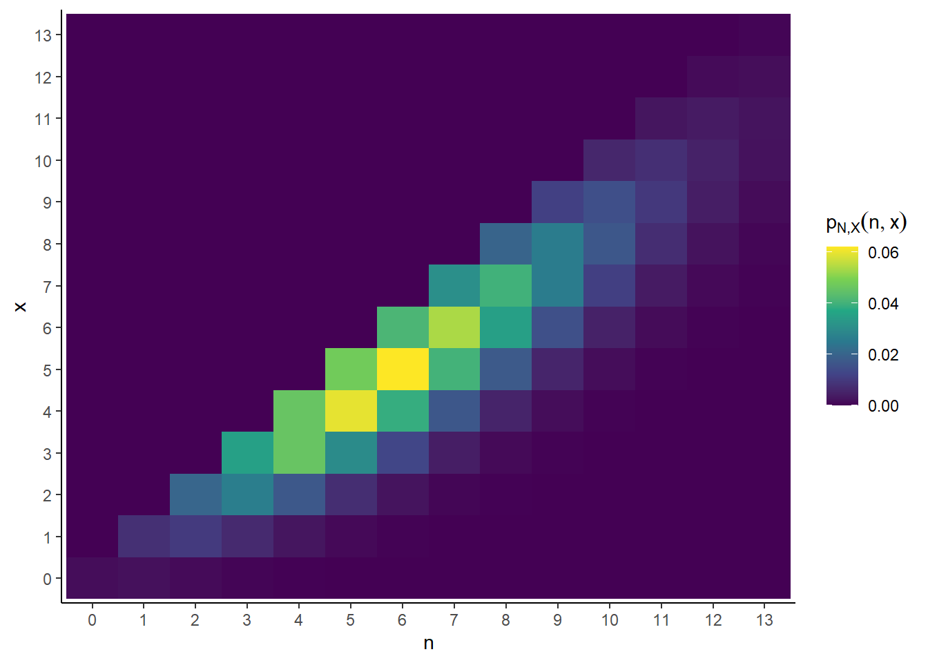
Figure 4.27: Tile plot representing the joint distribution of \(N\) and \(X\) in the chicken and egg problem in Example 4.34.
In the previous example we constructed the joint distribution using the general relationship \[ \text{joint} = \text{conditional}\times\text{marginal} \] We’ll study conditional distributions in more detail in the next section.
Be sure to distinguish between joint and marginal distributions.
- The joint distribution is a distribution on \((X, Y)\) pairs. A mathematical expression of a joint distribution is a function of both values of \(X\) and values of \(Y\). Pay special attention to the possible values; the possible values of one variable might be restricted by the value of the other.
- The marginal distribution of \(Y\) is a distribution on \(Y\) values only, regardless of the value of \(X\). A mathematical expression of a marginal distribution will have only values of the single variable in it; for example, an expression for the marginal distribution of \(Y\) will only have \(y\) in it (no \(x\), not even in the possible values).
4.7.2 Joint probability density fuctions
Recall that the joint distribution of random variables \(X\) and \(Y\) (defined on the same probability space) is a probability distribution on \((x, y)\) pairs. The joint distribution of two continuous random variables can be specified by a joint pdf, a surface specifying the density of \((x, y)\) pairs. The probability that the \((X,Y)\) pair of random variables lies is some region is the volume under the joint pdf surface over the region.
Bivariate Normal distributions are one commonly used family of joint continuous distribution. For example, the following plots represent the joint pdf surface of the Bivariate Normal distribution in the meeting problem in Section 2.12.1, with correlation 0.7.
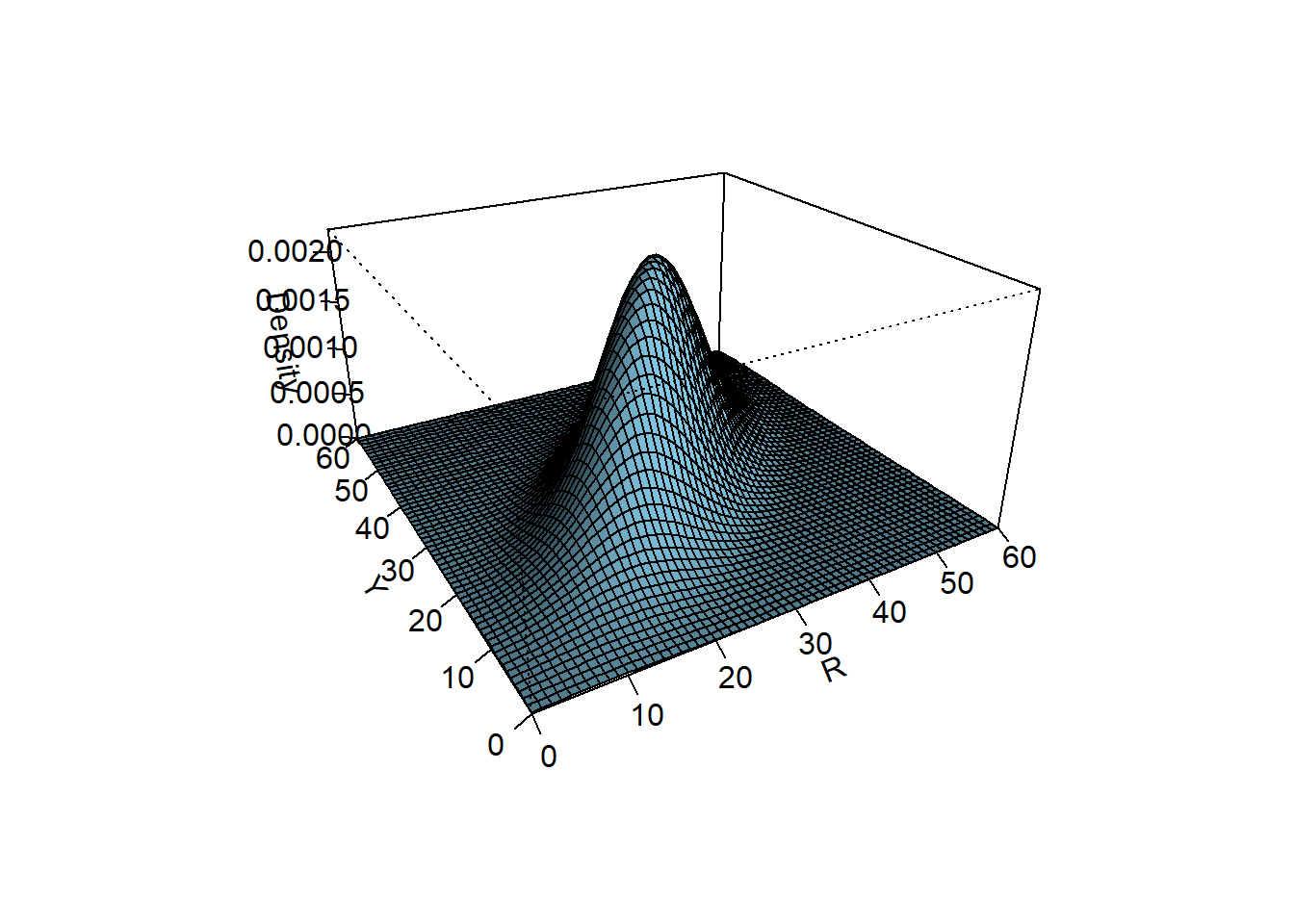
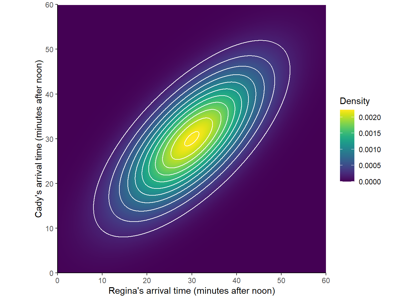
Figure 4.28: A Bivariate Normal distribution
Example 4.35 Suppose that
- \(X\) has a Normal(0, 1) distribution
- \(U\) has a Uniform(-2, 2) distribution
- \(X\) and \(U\) are generated independently
- \(Y = UX\).
Sketch a plot representing the joint pdf of \(X\) and \(Y\). Be sure to label axes with appropriate values.
Solution. to Example 4.35
Show/hide solution
Since \(X\) and \(Y\) are two continuous random variables, a scatterplot or joint density plot is appropriate. First identify possible values.
Since \(X\) has a Normal(0, 1) distribution, almost all of the values of \(X\) will fall between -3 and 3, so we can label the \(X\) axis from -3 to 3. (Or -2 to 2 is also fine for a sketch.)
The value of \(Y\) depends on both \(X\) and \(U\). For example, if \(X = 2\) then \(Y=2U\). Since \(U\) has a Uniform distribution, so does \(2U\), in particular, \(2U\) has a Uniform(-4, 4) distribution, so \(Y\) must be between -4 and 4 if \(X = 2\); similarly if \(X = -2\). In general, if \(X=x\) then \(Y\) has a Uniform(\(-2|x|\), \(2|x|\)) distribution, so larger values of \(|X|\) correspond to more extreme values of \(Y\). Since most values of X lie between -3 and 3, most values of Y lie between -6 and 6, so we can label the Y axis from -6 to 6. (Or -4 to 4 for a sketch.)
But as noted above, not all (X, Y) pairs are possible; only pairs within the region bounded by the lines \(y=2x\) and \(y=-2x\) have nonzero density.
Because \(X\) has a marginal Normal(0, 1) distribution, values of \(X\) near 0 are more likely, and values far from 0 are less likely. Within each vertical strip corresponding to an \(x\) value, the Y values are distributed uniformly between \(-2|x|\) and \(2|x|\). So as we move away from \(x=0\), the density height along each vertical strip between \(-2x\) and \(2x\) decreases, both because values away from 0 are less likely, and because the density is stretched thinner over longer vertical strips.
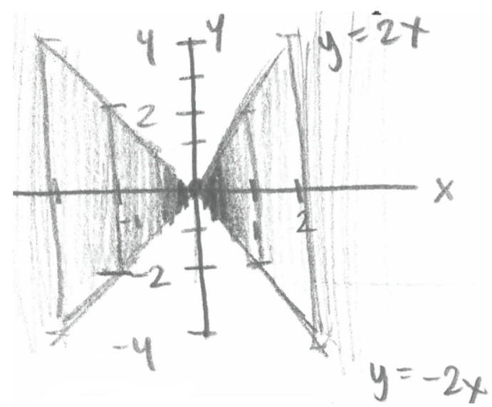
Figure 4.29: Hand sketch of a plot representing the joint pdf in 4.35
Here are a few questions to ask yourself when sketching plots.
- What is one possible plot point? A few possible points? It can often be difficult to know where to start, so just identifying a few possibilities can help.
- What type of plot is appropriate? Depends on the number (one or two) and types (discrete or continuous) of random variables involved.
- What are the possible values of the random variable(s)? After you answer this question you can start labeling your variable axes. For two random variables, be sure to identify possible pairs of values; identify the regions in the plot corresponding to possible pairs.
- What ranges of values are more likely? Less likely? The first few questions help you get a solid skeleton of a plot. Now you can start to sketch the shape of the distribution.
Definition 4.10 The joint probability density function (pdf) of two continuous random variables \((X,Y)\) defined on a probability space with probability measure \(\textrm{P}\) is the function \(f_{X,Y}:\mathbb{R}^2\mapsto[0,\infty)\) which satisfies, for any \(S\subseteq \mathbb{R}^2\), \[ \textrm{P}[(X,Y)\in S] = \iint\limits_{S} f_{X,Y}(x,y)\, dx dy \]
A joint pdf is a probability distribution on \((x, y)\) pairs. A joint pdf is a surface with height \(f_{X,Y}(x,y)\) at \((x, y)\). The probability that the \((X,Y)\) pair of random variables lies in the region \(A\) is the volume under the pdf surface over the region \(A\)
.)](_graphics/socr-bvn.PNG)
.)](_graphics/socr-bvn2.PNG)
Figure 4.30: (Left) A joint pdf. (Right) Volume under the surface represents probability. (Images from the SOCR Bivariate Normal distribution applet.)
A valid joint pdf must satisfy \[\begin{align*} f_{X,Y}(x,y) & \ge 0\\ \int_{-\infty}^\infty\int_{-\infty}^\infty f_{X,Y}(x,y)\, dx dy & = 1 \end{align*}\] Given a specific pdf, the generic bounds \((-\infty, \infty)\times(-\infty, \infty)\) in the above integral should be replaced by the range of possible pairs of values, that is, those \((x, y)\) pairs for which \(f_{X, Y}(x, y)>0\).
Recall that density is not probability. The height of the density surface at a particular \((x,y)\) pair is related to the probability that \((X, Y)\) takes a value “close to118” \((x, y)\) \[ \textrm{P}(x-\epsilon/2<X < x+\epsilon/2,\; y-\epsilon/2<Y < y+\epsilon/2) = \epsilon^2 f_{X, Y}(x, y) \qquad \text{for small $\epsilon$} \]
We now consider a continuous analog of rolling two fair four-sided dice. Instead of rolling a die which is equally likely to take the values 1, 2, 3, 4, we spin a Uniform(1, 4) spinner that lands uniformly in the continuous interval \([1, 4]\). When studying continuous random variables, it is often helpful to think about how a discrete analog behaves. So take a minute to recall the joint and marginal distributions of \(X\) and \(Y\) in the dice rolling example before proceeding.
Example 4.36 Spin the Uniform(1, 4) spinner twice, and let \(X\) be the sum of the two spins, and \(Y\) the larger spin (or the common value if there is a tie).
- Identify the possible values of \(X\), the possible values of \(Y\), and the possible \((X, Y)\) pairs. (Hint: think about the possible values of the spins and how \(X\) and \(Y\) are defined.)
- If \(U_1\) and \(U_2\) are the results of the two spins, explain why \(\text{P}(U_1 = U_2) = 0\).
- Explain intuitively why the joint density is constant over the region of possible \((X, Y)\) pairs. (Hint: compare to the discrete four-sided die case. There the probability of \((x, y)\) pairs was 2/16 for most possible pairs, because there were two pairs of rolls associated with each \((x, y)\) pair, e.g., rolls of (3, 2) or (2, 3) yield (5, 4) for \((X, Y)\). The exception was the \((x, y)\) pairs with probability 1/16 which correspond to rolling doubles, e.g. roll of (2, 2) yield (4, 2) for \((X, Y)\). Explain why we don’t need to worry about treating doubles as a separate case with the Uniform(1, 4) spinner.)
- Sketch a plot of the joint pdf.
- Find the joint pdf of \((X, Y)\).
- Use geometry to find \(\textrm{P}(X <4, Y > 2.5)\).
Solution. to Example 4.36
Show/hide solution
- Marginally, \(X\) takes values in \([2, 8]\) and \(Y\) takes values in \([1, 4]\). However, not every value in \([2, 8]\times [1, 4]\) is possible.
- We must have \(Y \ge 0.5 X\), or equivalently, \(X \le 2Y\). For example, if \(X=4\) then \(Y\) must be at least 2, because if the larger of the two spins were less than 2, then both spins must be less than 2, and the sum must be less than 4.
- We must have \(Y \le X - 1\), or equivalently, \(X \ge Y + 1\). For example, if \(Y=3\), then one of the spins is 3 and the other one is at least 1, so the sum must be at least 4.
- So the possible \((x, y)\) pairs must satisfy \(0.5x \le y \le x-1\) (or equivalently \(y +1\le x \le 2y\)), as well as \(2\le x\le8\) and \(1\le y \le 4\)
- \(\text{P}(U_1 = U_2) = 0\) because \(U_1\) and \(U_2\) are continuous (and independent). Whatever \(U_1\) is, say 2.35676355643243455…, the probability that \(U_2\) equals that value, with infinite precision, is 0.
- In the four-sided-die rolling situation there are basically two cases. Each \((X, Y)\) pair that correspond to a tie — that is each \((X, Y)\) pair with \(X = 2Y\) — has probability 1/16 (rolls of (1, 1), (2, 2), (3, 3), (4, 4). Each of the other possible \((X, Y)\) pairs has probability 2/16. In our continuous situation, consider a single \((X, Y)\) pair, say (5.7, 3.1). There are two outcomes — that is, pairs of spins — for which \(X=5.7, Y=3.1\), namely (3.1, 2.6) and (2.6, 3.1). Like (5.7, 3.1), most of the possible \((X, Y)\) values correspond to exactly two outcomes. The only ones that do not are the values with \(Y = 0.5X\) that lie along the south/east border of the triangular region. The pairs \((X, 0.5X)\) only correspond to exactly one outcome. For example, the only outcome corresponding to (6, 3) is the \((U_1, U_2)\) pair (3, 3); that is, the only way to have \(X=6\) and \(Y=3\) is to spin 3 on both spins. But because of the previous part, we don’t really need to worry about the ties as we did in the discrete case. Excluding ties, roughly, each pair in the triangular region of possible \((X, Y)\) pairs corresponds to exactly two outcomes (pairs of spins), and since the outcomes are uniformly distributed (over \([1, 4]\times[1, 4]\)) then the \((X, Y)\) pairs are also uniformly distributed (over the triangular region of possible values).
- See Figure 4.31. The joint density is constant over the triangular region of possible values. The plot provided is really a three-dimensional plot. The base is the triangular region which represents the possible \((X, Y)\) pairs. There is a surface floating above this region which has constant height.
- The joint density of \((X, Y)\) is constant over the range of possible values. The region \(\{(x, y): 2<x<8, 1<y<4, x/2<y<x-1\}\) is a triangle with area 4.5. The joint pdf is a surface of constant height floating above this triangle. The volume under the density surface is the volume of this triangular “wedge”. If the constant height is \(1/4.5 = 2/9\approx 0.222\), then the volume under the surface will be 1. Therefore, the joint pdf of \((X, Y)\) is \[ f_{X, Y}(x, y) = \begin{cases} 2/9, & 2<x<8,\; 1<y<4,\; x/2<y<x-1,\\ 0, & \text{otherwise} \end{cases} \]
- \(\textrm{P}(X <4, Y > 2.5) = 1/36\). The probability is the volume under the pdf over the region of interest. The base of the triangular wedge is \(\{(x, y): 3.5<x<4, 2.5<y<3, x/2<y\}\), a region which has area \((1/2)(4-3.5)(3-2.5) = 1/8\). Therefore, the volume of the triangular wedge that has constant height 2/9 is \((2/9)(1/8) = 1/36\).
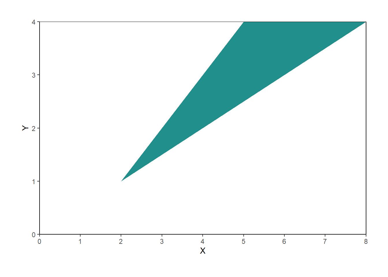
Figure 4.31: Joint distribution of \(X\) (sum) and \(Y\) (max) of two spins of the Uniform(1, 4) spinner. The triangular region represents the possible values of \((X, Y)\) the height of the density surface is constant over this region and 0 outside of the region.
Marginal pdfs can be obtained from the joint pdf by the law of total probability. In the discrete case, to find the marginal probability that \(X\) is equal to \(x\), sum the joint pmf \(p_{X, Y}(x, y)\) over all possible \(y\) values. The continuous analog is to integrate the joint pdf \(f_{X,Y}(x,y)\) over all possible \(y\) values to find the marginal density of \(X\) at \(x\). This can be thought of as “stacking” or “collapsing” the joint pdf.
\[\begin{align*} f_X(x) & = \int_{-\infty}^\infty f_{X,Y}(x,y) dy & & \text{a function of $x$ only} \\ f_Y(y) & = \int_{-\infty}^\infty f_{X,Y}(x,y) dx & & \text{a function of $y$ only} \end{align*}\]
The marginal distribution of \(X\) is a distribution on \(x\) values only. For example, the pdf of \(X\) is a function of \(x\) only (and not \(y\)). (Similarly the pdf of \(Y\) is a function of \(y\) only and not \(x\).)
In general the marginal distributions do not determine the joint distribution, unless the RVs are independent. In terms of a table: you can get the totals from the interior cells, but in general you can’t get the interior cells from the totals.
Example 4.37 Continuing Example 4.36. Spin the Uniform(1, 4) spinner twice, and let \(X\) be the sum of the two spins, and \(Y\) the larger spin.
- Sketch a plot of the marginal distribution of \(Y\). Be sure to specify the possible values.
- Suggest an expression for the marginal pdf of \(Y\).
- Use calculus to derive \(f_Y(2.5)\), the marginal pdf of \(Y\) evaluated at \(y=2.5\).
- Use calculus to derive \(f_Y\), the marginal pdf of \(Y\).
- Find \(\textrm{P}(Y > 2.5)\).
- Sketch a plot of the marginal distribution of \(X\). Be sure to specify the possible values. (Hint: think “collapsing/stacking” the joint distribution; compare with the dice rolling example.)
- Suggest an expression for the marginal pdf of \(X\).
- Use calculus to derive \(f_X(4)\), the marginal pdf of \(X\) evaluated at \(x=4\).
- Use calculus to derive \(f_X(6.5)\), the marginal pdf of \(X\) evaluated at \(x=6.5\).
- Use calculus to derive \(f_X\), the marginal pdf of \(X\). Hint: consider \(x<5\) and \(x>5\) separately.
- Find \(\textrm{P}(X < 4)\).
- Find \(\textrm{P}(X < 6.5)\).
Solution. to Example 4.37
Show/hide solution
- Marginally, the possible values of \(Y\) are [1, 4]. For each possible \(y\), “collapse out” the \(X\) values by “stacking” each horizontal slice. Density will be smallest at 1 and highest at 4; see the plot below and compare to the positively sloped impulse plot in the dice rolling case.
- Density is 0 at \(y=1\) increasing to a maximum at \(y=4\). If we assume that the marginal density of \(Y\) is linear in \(y\) (similar to the discrete dice rolling case), with a height of 0 at \(y=1\) at a height of \(c\) at \(y=4\), we might guess \[ f_Y(y) = \begin{cases} c(y - 1), & 1<y<4,\\ 0, & \text{otherwise.} \end{cases} \] Then find \(c\) to make the total area under the pdf equal 1. The area under the pdf is the area of a triangle with base 4-1 and height \(c(4-1)\) so setting \(1=(1/2)(4-1)(c(4-1))\) yields \(c=2/9\). \[ f_Y(y) = (2/9)(y-1), \qquad 1<y<4 \] We confirm below that this is the marginal pdf of \(Y\).
- We find the marginal pdf of \(Y\) evaluated at \(y=2.5\) by “stacking” the density at each pair \((x, 2.5)\) over the possible \(x\) values. For discrete variables, the stacking is achieved by summing the joint pmf over the possible \(x\) values. For continuous random variables we integrate the joint pdf over the possible \(x\) values corresponding to \(y=2.5\). If \(y=2.5\) then \(3.5 < x< 5\). “Integrate out the \(x\)’s” by computing a \(dx\) integral: \[ f_Y(2.5) = \int_{3.5}^5 (2/9)\, dx = (2/9)x \Bigg|_{x=3.5}^{x=5} = 1/3 \] This agrees with the result of plugging in \(y=2.5\) in the expression in the previous part.
- To find the marginal pdf of \(Y\) we repeat the calculation from the previous part for each possible value of \(y\). Fix a \(1<y<4\), and replace 2.5 in the previous part with a generic \(y\). The possible values of \(x\) corresponding to a given \(y\) are \(y + 1 < x < 2y\). “Integrate out the \(x\)’s” by computing a \(dx\) integral. Within the \(dx\) integral, \(y\) is treated like a constant. \[ f_Y(y) = \int_{y+1}^{2y} (2/9)\, dx = (2/9)x \Bigg|_{x=y+1}^{x=2y} = (2/9)(y-1), \qquad 1<y<4 \] Thus, we have confirmed that our suggested form of the marginal pdf is correct.
- If we have already derived the marginal pdf of \(Y\), we can treat this just like a one variable problem. Integrate the pdf of \(Y\) over \((2.5, 4)\) \[ \textrm{P}(Y > 2.5) = \int_{2.5}^4 (2/9)(y-1)\, dy = (1/9)(y-1)^2\Bigg|_{y=2.5}^{y=4} = 0.25 \] (Integration is not really needed; instead, sketch a picture and use geometry.)
- Marginally, the possible values of \(X\) are [2, 8]. For each possible \(x\), “collapse out” the \(Y\) values by “stacking” each vertical slice. Density will be smallest at 2 and 8 and highest at 5; see the plot below and compare to the triangular impulse plot in the dice rolling case.
- We see that the density is 0 at \(x=2\) and \(x=8\) and has a triangular shape with a peak at \(x=5\). If \(c\) is the density at \(x=5\), then \(1 = (1/2)(8-2)c\) implies \(c=1/3\). We might guess \[ f_X(x) = \begin{cases} (1/9)(x-2), & 2 < x< 5,\\ (1/9)(8-x), & 5<x<8,\\ 0, & \text{otherwise.} \end{cases} \] We could also write this as \(f_X(x) = 1/3 - (1/9)|x - 5|, 2<x<8\). We confirm below that this is the marginal pdf of \(X\).
- We find the marginal pdf of \(X\) evaluated at \(x=4\) by “stacking” the density at each pair \((4, y)\) over the possible \(y\) values. For discrete variables, the stacking is achieved by summing the joint pmf over the possible \(y\) values. For continuous random variables we integrate the joint pdf over the possible \(y\) values corresponding to \(x=4\). If \(x=4\) then \(2 < y< 3\). “Integrate out the \(y\)’s” by computing a \(dy\) integral: \[ f_X(4) = \int_{2}^3 (2/9)\, dy = (2/9)y \Bigg|_{y=2}^{y=3} = 2/9 \approx 0.222 \] This agrees with the result of plugging in \(x=4\) in the expression in the previous part.
- This is similar to the previous part, but for \(x=6.5\), we hit the upper bound of 4 on \(y\) values; that is, the range isn’t just from \(x/2\) to \(x-1\), but rather \(x/2\) to 4. If \(x=6.5\) then \(3.25 < y< 4\). “Integrate out the \(y\)’s” by computing a \(dy\) integral: \[ f_X(6.5) = \int_{3.25}^4 (2/9)\, dy = (2/9)y \Bigg|_{y=3.25}^{y=4} = 1/6 \approx 0.167 \] This agrees with the result of plugging in \(x=6.5\) in the expression in two parts ago.
- For \(2<x<5\) the bounds on possible \(y\) values are \(x/2\) to \(x-1\) \[ f_X(x) = \int_{x/2}^{x-1} (2/9)\, dy = (2/9)y \Bigg|_{y=x/2}^{y=x-1} = (1/9)(x - 2), \qquad 2<x<5. \] For \(5<x<8\) the bounds on possible \(y\) values are \(x/2\) to \(4\) \[ f_X(x) = \int_{x/2}^{4} (2/9)\, dy = (2/9)y \Bigg|_{y=x/2}^{y=4} = (1/9)(8 - x), \qquad 5<x<8. \] So the calculus matches what we did a few parts ago.
- If we have already derived the marginal pdf of \(X\), we can treat this just like a one variable problem. Integrate the pdf of \(X\) over \((2, 4)\) \[ \textrm{P}(X < 4) = \int_{2}^4 (1/9)(x-2)\, dx = (1/18)(x-2)^2\Bigg|_{x=2}^{x=4} = 2/9 \approx 0.222 \] (Integration isn’t really needed here; instead, sketch a picture and use geometry.)
- If we have already derived the marginal pdf of \(X\), we can treat this just like a one variable problem. It’s easiest to use the complement rule and integrate the pdf of \(X\) over \((6.5, 8)\) \[ \textrm{P}(X < 6.5) = 1 - \textrm{P}(X > 6.5) = 1 - \int_{6.5}^8 (1/9)(8-x)\, dx =1 - (-1/18)(8-x)^2\Bigg|_{x=6.5}^{x=8} = 1 - 1/8 = 7/8 = 0.875 \] (Integration isn’t really needed here; instead, sketch a picture and use geometry.)
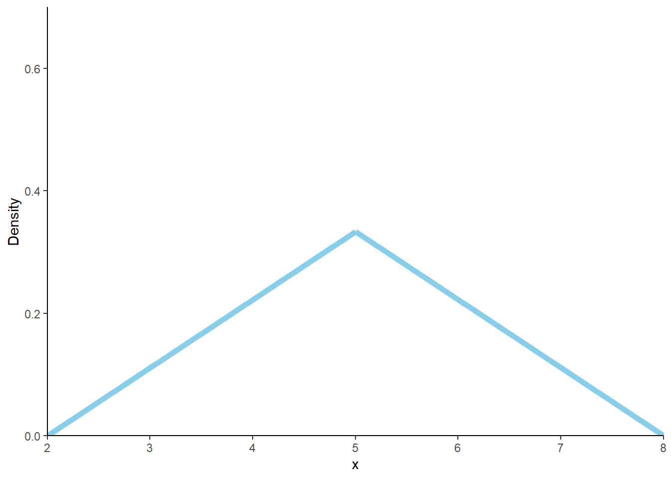
Figure 4.32: Marginal distribution of \(X\), the sum of two spins of a Uniform(1, 4) spinner.
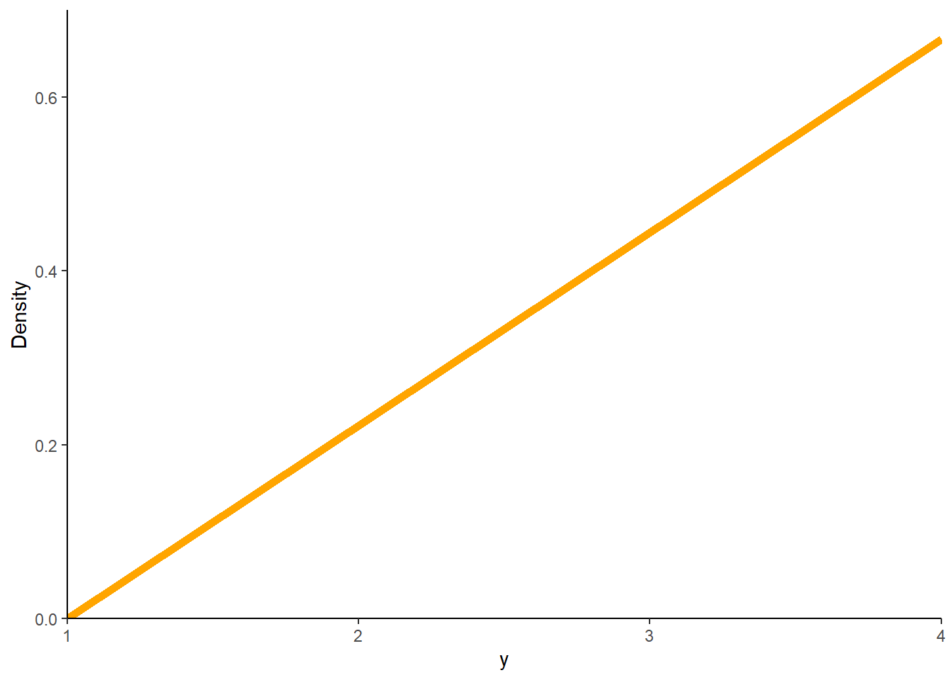
Figure 4.33: Marginal distribution of \(Y\), the larger of two spins of a Uniform(1, 4) spinner.
Example 4.38 Let \(X\) be the time (hours), starting now, until the next earthquake (of any magnitude) occurs in SoCal, and let \(Y\) be the time (hours), starting now, until the second earthquake from now occurs (so that \(Y-X\) is the time between the first and second earthquake). Suppose that \(X\) and \(Y\) are continuous RVs with joint pdf
\[ f_{X, Y}(x, y) = \begin{cases} 4e^{-2y}, & 0 < x< y < \infty,\\ 0, & \text{otherwise} \end{cases} \]
- Is the joint pdf a function of both \(x\) and \(y\)? How?
- Why is \(f_{X, Y}(x, y)\) equal to 0 if \(y < x\)?
- Sketch a plot of the joint pdf. What does its shape say about the distribution of \(X\) and \(Y\) in this context?
- Set up the integral to find \(\textrm{P}(X > 0.5, Y < 1)\).
Solution. to Example 4.38
Show/hide solution
- Yes, the pdf is a function of both \(x\) and \(y\). Pay attention to the possible values. We need to know both \(x\) and \(y\) to determine if the density is 0 or not.
- \(X\) is the time from now until the the first earthquake and \(Y\) is the time from now until the second, so we must have \(Y \ge X\) since the second can’t happen before the first!
- The density is 0 below the line \(y = x\). Given any \(x\) value, the density over each vertical strip is highest at \(y = x\) and then decreases exponentially as \(y\) increases. Given any \(y\), the density is constant along the horizontal strip between 0 and \(x = y\). Since as \(y\) increases the range of corresponding possible \(x\) values — 0 to \(x = y\) — increases, the density along each horizontal strip gets stretched over longer regions, so the constant height decreases as \(y\) increases. The density will be highest for pairs where the time until the first earthquake is close to 0, and the second earthquake occurs soon after the first. See Figure 4.34.
- We will see easier ways of doing this later. But in principle, \(\textrm{P}(X > 0.5, Y < 1)\) is the volume under the joint pdf over the triangular region \(\{x>0.5, y < 1, x < y\}\). The integral is a double integral; you can integrate either \(dx\) or \(dy\) first, but careful about the bounds on the integrals. \[ \int_{0.5}^1\left(\int_x^1 4e^{-2y}dy\right)dx = \int_{0.5}^1 4e^{-2y}\left(\int_{0.5}^{y}dx\right)dy = 0.097 \] For about 9.7% of earthquakes the next two earthquakes happen between 30 minutes and 1 hour later.
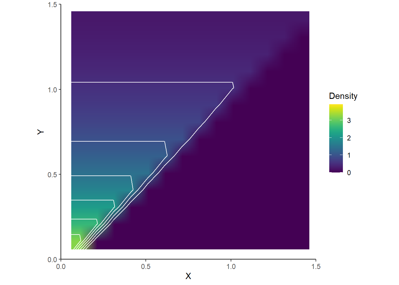
Figure 4.34: Heat map representing the joint pdf of \(X\) and \(Y\) in Example 4.38.
Example 4.39 Continuing Example 4.38. Let \(X\) be the time (hours), starting now, until the next earthquake (of any magnitude) occurs in SoCal, and let \(Y\) be the time (hours), starting now, until the second earthquake from now occurs (so that \(Y-X\) is the time between the first and second earthquake). Suppose that \(X\) and \(Y\) are continuous RVs with joint pdf
\[ f_{X, Y}(x, y) = \begin{cases} 4e^{-2y}, & 0 < x< y < \infty,\\ 0, & \text{otherwise} \end{cases} \]
- Sketch a plot of the marginal pdf of \(X\). Be sure to specify possible values.
- Find the marginal pdf of \(X\) at \(x=0.5\).
- Find the marginal pdf of \(X\). Be sure to specify possible values. Identify the marginal distribution of \(X\) be name.
- Compute and interpret \(\textrm{P}(X > 0.5)\).
- Sketch the marginal pdf of \(Y\). Be sure to specify possible values.
- Find the marginal pdf of \(Y\) at \(y=1.5\).
- Find the marginal pdf of \(Y\). Be sure to specify possible values of \(Y\).
- Compute and interpret find \(\textrm{P}(Y < 1)\).
- Is \(\textrm{P}(X > 0.5, Y < 1)\) equal to the product of \(\textrm{P}(X > 0.5)\) and \(\textrm{P}(Y < 1)\)? Why?
Solution. to Example 4.39
Show/hide solution
- See Figure 4.35. Marginally \(X\) can take any positive value. Collapse out the \(Y\) values in the joint pdf. The vertical strips corresponding to \(x\) near 0 are the longest and have the highest density. So when the vertical strips are collapsed the marginal density will be highest at \(x=0\) and decrease as \(x\) increases.
- Collapse the vertical strip corresponding to \(x=0.5\) by integrating out the \(y\) values; if \(x = 0.5\) then density is positive for \(y>0.5\). \[ f_X(0.5) = \int_{0.5}^\infty 4e^{-2y}dy = 2e^{-2(0.5)} \]
- Repeat the previous part with 0.5 replaced by a generic \(x>0\). \[ f_X(x) = \int_{x}^\infty 4e^{-2y}dy = 2e^{-2x} \] \(X\) has an Exponential distribution with rate parameter 2.
- Once we have the marginal pdf of \(X\) we can integrate as usual. But we can also use properties of Exponential distributions: \(\textrm{P}(X>0.5) = e^{-2(0.5)}=0.368\) For about 36.8% of earthquakes the next earthquake occurs after 30 minutes.
- See Figure 4.36. Marginally \(Y\) can take any positive value. Collapse out the \(X\) values in the joint pdf. There are two features at work. The horizontal strips corresponding to \(y\) near 0 are the shortest, but they have the highest density. As \(y\) increases, the corresponding horizontal strips get longer, but lower. It’s hard to tell exactly what the shape will be when the horizontal strips are collapsed, but one guess is that the marginal density will start low at \(y=0\), then increase over some range of \(y\) values, but then decrease again.
- Collapse the vertical strip corresponding to \(y=1.5\) by integrating out the \(x\) values; if \(y = 1.5\) then density is positive for \(x<1.5\). \[ f_Y(1.5) = \int_{0}^{1.5} 4e^{-2(1.5)}dx = 4(1.5)e^{-2(1.5)} \]
- Repeat the previous part with 1.5 replaced by a generic \(y>0\). \[ f_Y(y) = \int_{0}^y 4e^{-2y}dx = 4ye^{-2y} \] That is, the marginal pdf of \(Y\) is \(f_Y(y) = 4ye^{-2y}, y>0\). (This distribution is the “Gamma” distribution with shape parameter 2 and rate parameter 2.).
- Once we have the marginal pdf of \(Y\) we can integrate it as usual \[ \textrm{P}(Y < 1) = \int_0^1 4y e^{-2y}dy = 0.594 \] For about 59.4% of earthquakes, at least two earthquakes happen within 2 hours.
- No, the joint probability is not equal to the product of the marginal probabilities because \(X\) and \(Y\) are not independent since we must have \(X\le Y\).
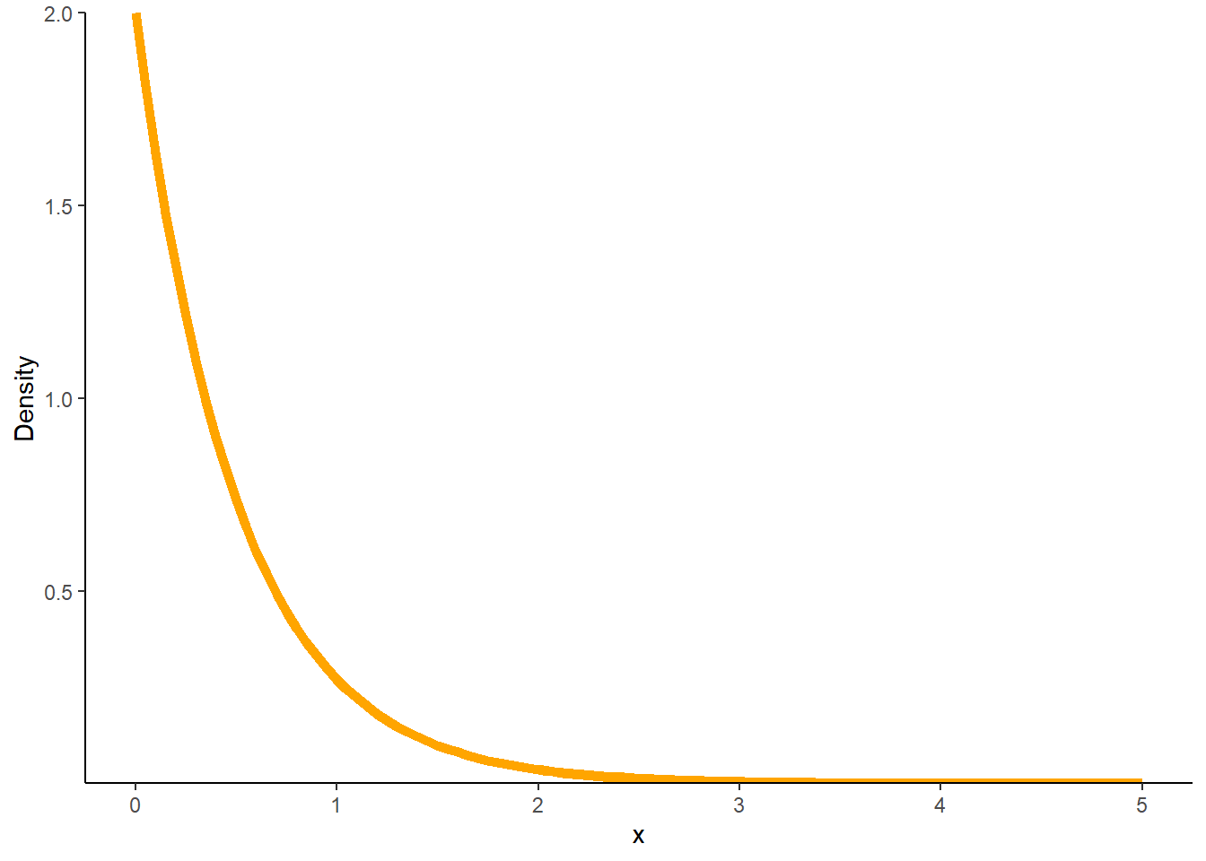
Figure 4.35: Marginal distribution of \(X\) in Example 4.39.
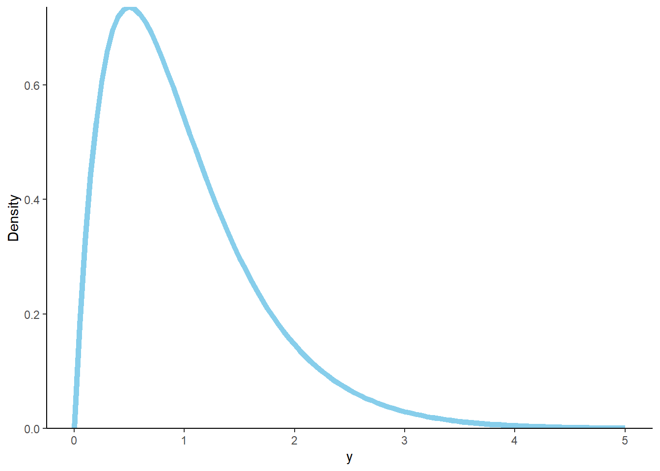
Figure 4.36: Marginal distribution of \(Y\) in Example 4.39.
Be sure to distinguish between joint and marginal distributions.
- The joint distribution is a distribution on \((X, Y)\) pairs. A mathematical expression of a joint distribution is a function of both values of \(X\) and values of \(Y\). Pay special attention to the possible values; the possible values of one variable might be restricted by the value of the other.
- The marginal distribution of \(Y\) is a distribution on \(Y\) values only, regardless of the value of \(X\). A mathematical expression of a marginal distribution will have only values of the single variable in it; for example, an expression for the marginal distribution of \(Y\) will only have \(y\) in it (no \(x\), not even in the possible values).
We mostly focus on the case of two random variables, but analogous definitions and concepts apply for more than two (though the notation can get a bit messier).↩︎
You can have different precisions for \(X\) and \(Y\), e.g., \(\epsilon_x, \epsilon_y\), but using one \(\epsilon\) makes the notation a little simpler.↩︎